
Install the app
How to install the app on iOS
Follow along with the video below to see how to install our site as a web app on your home screen.
Note: This feature may not be available in some browsers.
You are using an out of date browser. It may not display this or other websites correctly.
You should upgrade or use an alternative browser.
You should upgrade or use an alternative browser.
Ladik komt met een integrator module!!
- Thread starter ProgHead
- Start date

Voor de CV-modus vinden we dus:
[imath] \mathrm{gn}(\alpha) = \frac{ -180 \, \alpha^4 + 180 \, \alpha^3 + 900 \, \alpha^2 }{ 400 \, \alpha^5 + 1280 \, \alpha^4 - 5760 \, \alpha^3 - 6720 \, \alpha^2 +10800 \, \alpha + 2000 } \,\,\,\,\,\,\, (21) [/imath]
En met een online graph plotter:
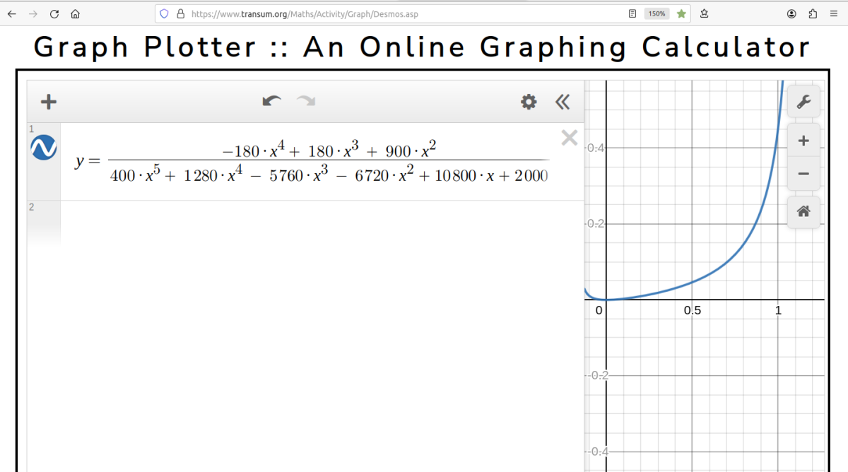
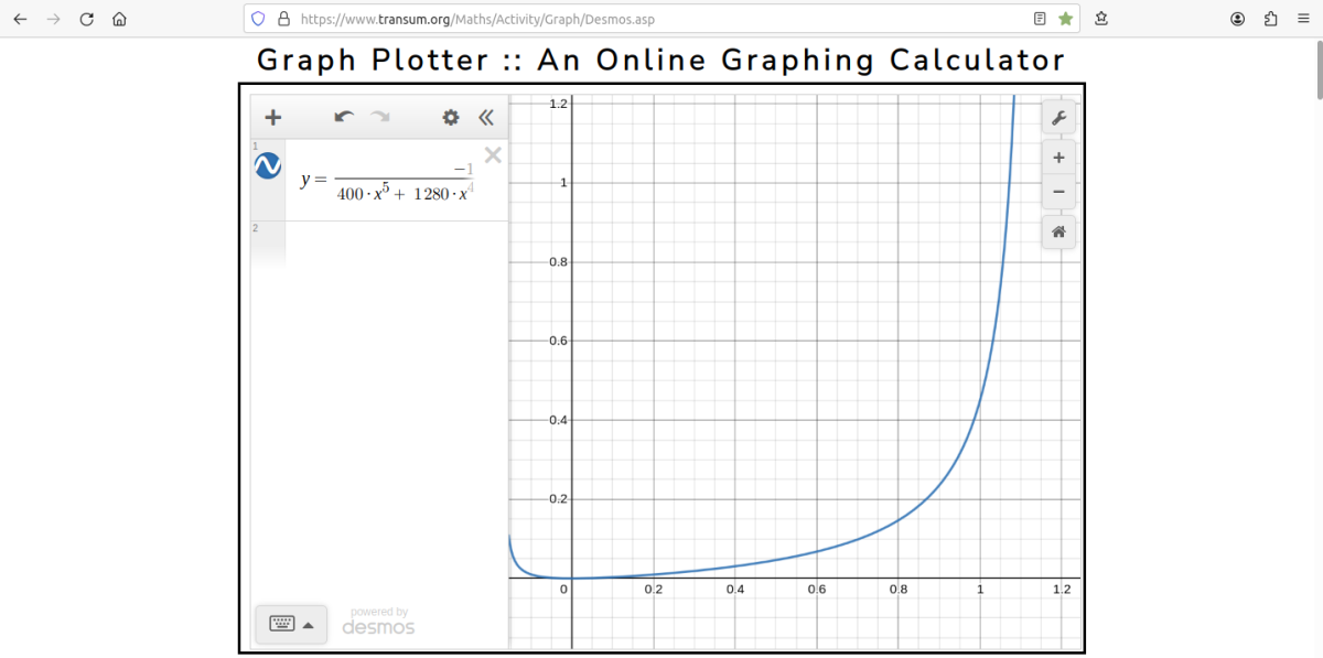
[imath] \mathrm{gn}(\alpha) = \frac{ -180 \, \alpha^4 + 180 \, \alpha^3 + 900 \, \alpha^2 }{ 400 \, \alpha^5 + 1280 \, \alpha^4 - 5760 \, \alpha^3 - 6720 \, \alpha^2 +10800 \, \alpha + 2000 } \,\,\,\,\,\,\, (21) [/imath]
En met een online graph plotter:
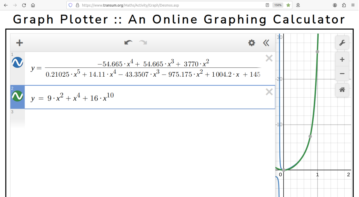
En voor de HI-modus:
[imath] \mathrm{gn}(\alpha) = \frac{ -54.665 \, \alpha^4 + 54.665 \, \alpha^3 + 3770 \, \alpha^2 }{ 0.21025 \, \alpha^5 + 14.11 \, \alpha^4 - 43.3507 \, \alpha^3 - 975.175 \, \alpha^2 + 1004.2 \, \alpha + 145 } \,\,\,\,\,\,\,\,\, (22) [/imath]
En met de online graph plotter:
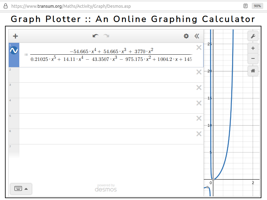
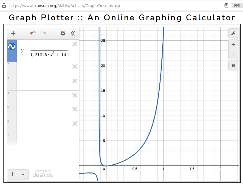
[imath] \mathrm{gn}(\alpha) = \frac{ -54.665 \, \alpha^4 + 54.665 \, \alpha^3 + 3770 \, \alpha^2 }{ 0.21025 \, \alpha^5 + 14.11 \, \alpha^4 - 43.3507 \, \alpha^3 - 975.175 \, \alpha^2 + 1004.2 \, \alpha + 145 } \,\,\,\,\,\,\,\,\, (22) [/imath]
En met de online graph plotter:
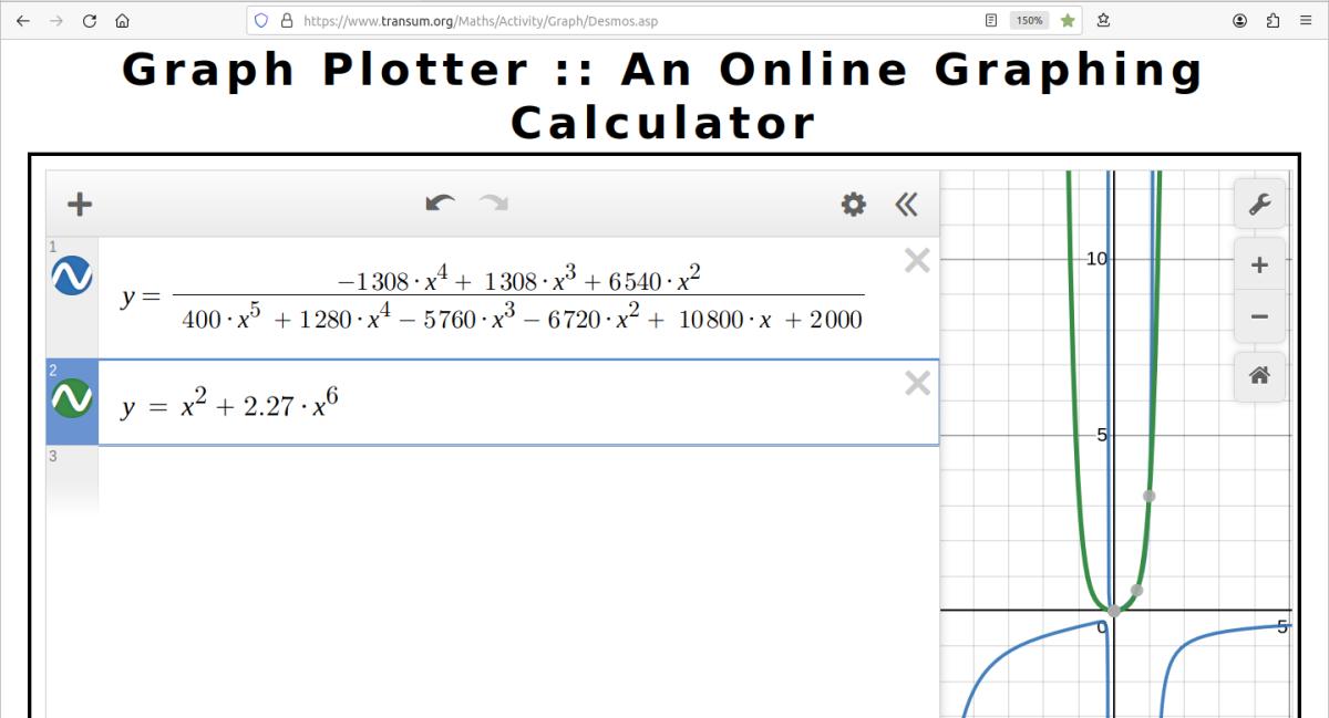
En ten slotte voor de LO-modus:
[imath] \mathrm{gn}(\alpha) = \frac{ -1308 \, \alpha^4 + 1308 \, \alpha^3 + \, 6540 \, \alpha^2 }{ 400 \, \alpha^5 + 1280 \, \alpha^4 - 5760 \, \alpha^3 - 6720 \, \alpha^2 + 10800 \, \alpha + 2000 } \,\,\,\,\,\,\,\,\, (23) [/imath]
En met de online graph plotter:
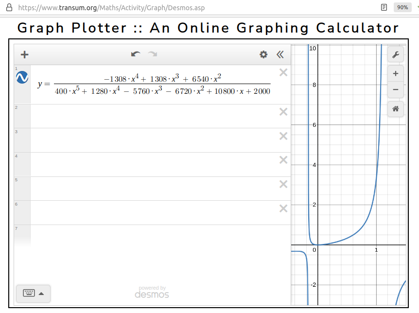
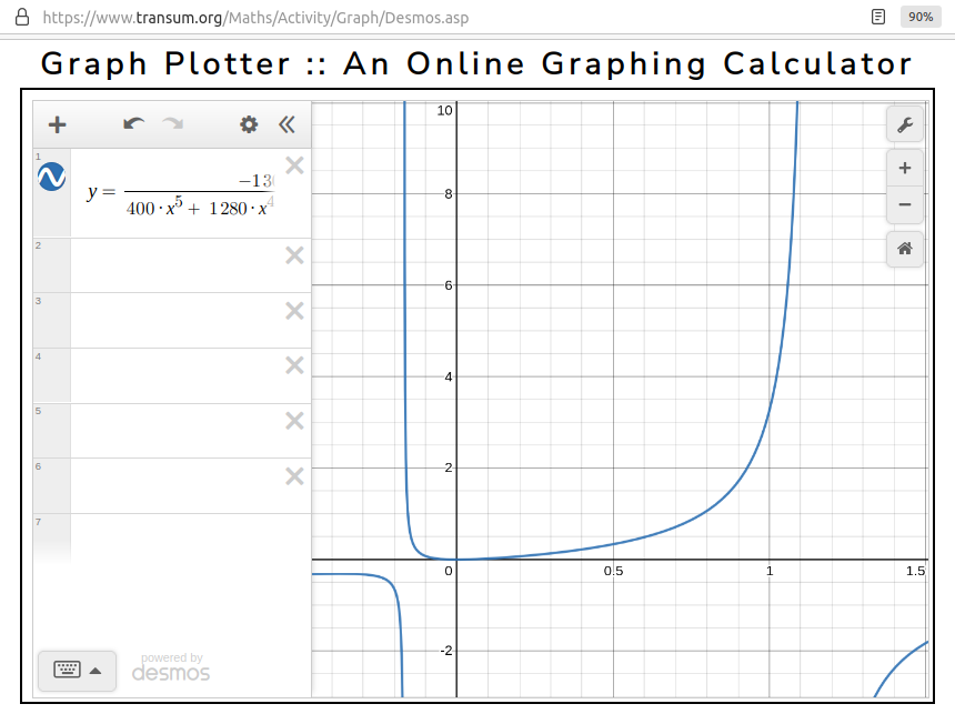
[imath] \mathrm{gn}(\alpha) = \frac{ -1308 \, \alpha^4 + 1308 \, \alpha^3 + \, 6540 \, \alpha^2 }{ 400 \, \alpha^5 + 1280 \, \alpha^4 - 5760 \, \alpha^3 - 6720 \, \alpha^2 + 10800 \, \alpha + 2000 } \,\,\,\,\,\,\,\,\, (23) [/imath]
En met de online graph plotter:
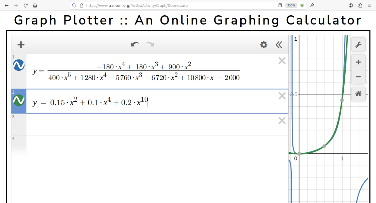
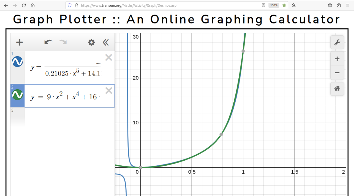
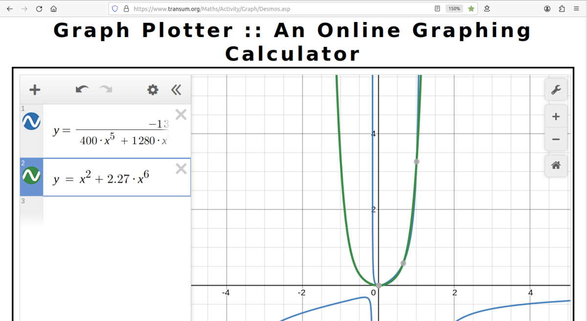
Met behulp van een online graph plotter heb ik zo juist simpele benaderende formules (24), (25) en (26) (zie hieronder) gevonden die gezien de toch al beperkte nauwkeurigheid van dit project probleemloos in plaats van de eerder gevonden nogal gecompliceerde formules (21), (22) en (23) kunnen worden gebruikt. Om verwarring te voorkomen schrijf ik in de nieuwe formules [imath] \mathrm{gn}^*( \,\, ) [/imath] in plaats van [imath] \mathrm{gn}( \,\, ) [/imath]. We hebben dan:
[imath] \mathrm{(CV)} \,\,\, \mathrm{gn}^*( \alpha ) = 0,15 \, \alpha^2 + 0,1 \, \alpha^4 + 0,2 \, \alpha^{10} \,\,\,\,\,\,\, (24) [/imath]
[imath] \mathrm{(HI)} \,\,\,\, \mathrm{gn}^*( \alpha ) = 9 \, \alpha^2 + \alpha^4 + 16 \, \alpha^{10} \,\,\,\,\,\,\, (25) [/imath]
[imath] \mathrm{(LO)} \,\,\,\, \mathrm{gn}^*( \alpha ) = \alpha^2 + 2,27 \, \alpha^6 \,\,\,\,\,\,\, (26) [/imath]
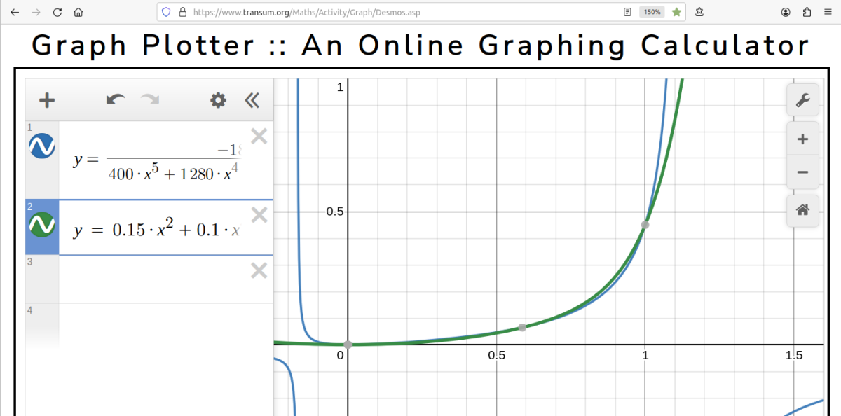
Bedenk dat [imath] 0 \leq \alpha \leq 1[/imath]. De onderstaande plaatjes laten zien hoe goed de benaderingen zijn:
CV
HI
LO
[imath] \mathrm{(CV)} \,\,\, \mathrm{gn}^*( \alpha ) = 0,15 \, \alpha^2 + 0,1 \, \alpha^4 + 0,2 \, \alpha^{10} \,\,\,\,\,\,\, (24) [/imath]
[imath] \mathrm{(HI)} \,\,\,\, \mathrm{gn}^*( \alpha ) = 9 \, \alpha^2 + \alpha^4 + 16 \, \alpha^{10} \,\,\,\,\,\,\, (25) [/imath]
[imath] \mathrm{(LO)} \,\,\,\, \mathrm{gn}^*( \alpha ) = \alpha^2 + 2,27 \, \alpha^6 \,\,\,\,\,\,\, (26) [/imath]
Bedenk dat [imath] 0 \leq \alpha \leq 1[/imath]. De onderstaande plaatjes laten zien hoe goed de benaderingen zijn:
CV
HI
LO
Waarschijnlijk al eens eerder afgeleid maar ik kan het niet meer vinden. Dus hier is die weer: de leaky inverting integrator.
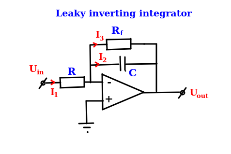
[imath] I_1 = \frac{U_{in}}{\mathrm{R}} [/imath]
[imath] I_2 = \mathrm{C}\, \frac{\mathrm{d} (-U_{out})}{ \mathrm{d} t} [/imath]
[imath] I_2 = - \mathrm{C}\, \frac{\mathrm{d} U_{out}}{ \mathrm{d} t} [/imath]
[imath] I_3 = \frac{- U_{out}}{\mathrm{R}_f} [/imath]
[imath] I_1 = I_2 + I_3 [/imath]
[imath] \frac{U_{in}}{\mathrm{R}} = - \mathrm{C}\, \frac{\mathrm{d} U_{out}}{ \mathrm{d} t} + \frac{- U_{out}}{\mathrm{R}_f} [/imath]
[imath] \frac{U_{in}}{\mathrm{R} \mathrm{C} } = - \frac{\mathrm{d} U_{out}}{ \mathrm{d} t} + \frac{- U_{out}}{\mathrm{R}_f \mathrm{C} } [/imath]
[imath] - \frac{U_{in}}{\mathrm{R} \mathrm{C} } = \frac{\mathrm{d} U_{out}}{ \mathrm{d} t} + \frac{U_{out}}{\mathrm{R}_f \mathrm{C} } [/imath]
Of anders geschreven:
[imath] - \frac{U_{in}}{\tau} = \frac{\mathrm{d} U_{out}}{ \mathrm{d} t} + \frac{U_{out}}{\tau_f} \,\,\,\,\,\, \mathrm{voor} \,\,\,\, \tau = \mathrm{R} \mathrm{C} \,\,\,\, \& \,\,\,\, \tau_f = \mathrm{R}_f \mathrm{C} \,\,\,\,\,\,\,\,\,\, (27) [/imath]
[imath] I_1 = \frac{U_{in}}{\mathrm{R}} [/imath]
[imath] I_2 = \mathrm{C}\, \frac{\mathrm{d} (-U_{out})}{ \mathrm{d} t} [/imath]
[imath] I_2 = - \mathrm{C}\, \frac{\mathrm{d} U_{out}}{ \mathrm{d} t} [/imath]
[imath] I_3 = \frac{- U_{out}}{\mathrm{R}_f} [/imath]
[imath] I_1 = I_2 + I_3 [/imath]
[imath] \frac{U_{in}}{\mathrm{R}} = - \mathrm{C}\, \frac{\mathrm{d} U_{out}}{ \mathrm{d} t} + \frac{- U_{out}}{\mathrm{R}_f} [/imath]
[imath] \frac{U_{in}}{\mathrm{R} \mathrm{C} } = - \frac{\mathrm{d} U_{out}}{ \mathrm{d} t} + \frac{- U_{out}}{\mathrm{R}_f \mathrm{C} } [/imath]
[imath] - \frac{U_{in}}{\mathrm{R} \mathrm{C} } = \frac{\mathrm{d} U_{out}}{ \mathrm{d} t} + \frac{U_{out}}{\mathrm{R}_f \mathrm{C} } [/imath]
Of anders geschreven:
[imath] - \frac{U_{in}}{\tau} = \frac{\mathrm{d} U_{out}}{ \mathrm{d} t} + \frac{U_{out}}{\tau_f} \,\,\,\,\,\, \mathrm{voor} \,\,\,\, \tau = \mathrm{R} \mathrm{C} \,\,\,\, \& \,\,\,\, \tau_f = \mathrm{R}_f \mathrm{C} \,\,\,\,\,\,\,\,\,\, (27) [/imath]
Even terug in de tijd (en daarmee naar het begin van ons bewijs  ):
):
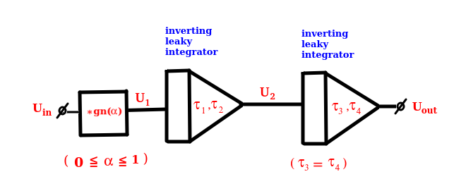
Het meest linkse blokje is al klaar. En een vergelijking voor de inverting leaky integrators hebben we ook al. Namelijk:
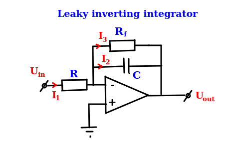
[imath] - \frac{U_{in}}{\tau} = \frac{\mathrm{d} U_{out}}{ \mathrm{d} t} + \frac{U_{out}}{\tau_f} \,\,\,\,\,\, \mathrm{voor} \,\,\,\, \tau = \mathrm{R} \mathrm{C} \,\,\,\, \& \,\,\,\, \tau_f = \mathrm{R}_f \mathrm{C} \,\,\,\,\,\,\,\,\,\, (27) [/imath]
Concreet ziet de Falstad simulatie er voor de drie modi zo uit:
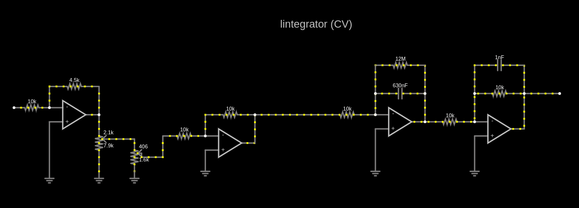
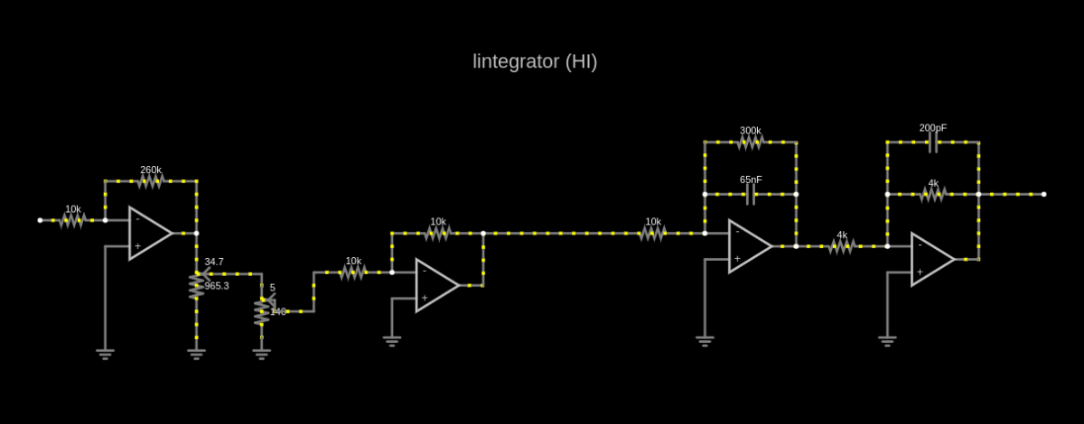
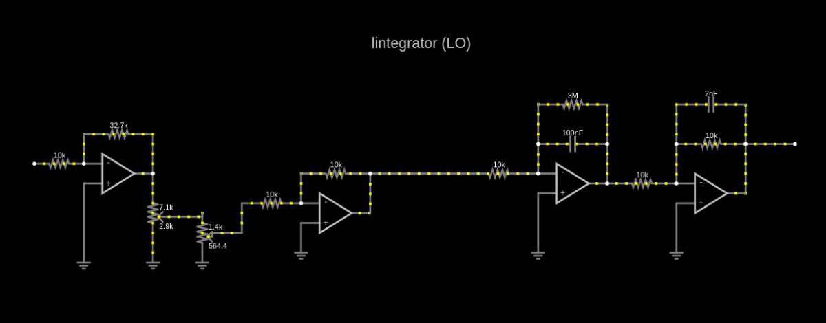
Waaruit we de tijdsconstanten [imath] \tau_1 [/imath] t/m [imath] \tau_4 [/imath] vinden voor de drie modi CV, HI en LO:
Voor CV: [imath] \tau_1 = 10 \mathrm{k}\Omega \cdot 630 \mathrm{nF} = 6,3 \mathrm{ms} \,\,\, \& \,\,\, \tau_2 = 12 \mathrm{M}\Omega \cdot 630 \mathrm{nF} = 7,56 \mathrm{s} \,\,\, \& \,\,\, \tau_3 = 10 \mathrm{k}\Omega \cdot 1 \mathrm{nF} = 10 \mu \mathrm{s} \,\,\, \& \,\,\, \tau_4 = 10 \mathrm{k}\Omega \cdot 1 \mathrm{nF} = 10 \mu \mathrm{s} \,\,\,\,\,\,\, (28) [/imath]
Voor HI: [imath] \tau_1 = 10 \mathrm{k}\Omega \cdot 65 \mathrm{nF} = 650 \mu \mathrm{s} \,\,\, \& \,\,\, \tau_2 = 300 \mathrm{k}\Omega \cdot 65 \mathrm{nF} = 19,5 \mathrm{ms} \,\,\, \& \,\,\, \tau_3 = 4 \mathrm{k}\Omega \cdot 200 \mathrm{pF} = 800 \mathrm{ns} \,\,\, \& \,\,\, \tau_4 = 4 \mathrm{k}\Omega \cdot 200 \mathrm{pF} = 800 \mathrm{ns} \,\,\,\,\,\,\, (29) [/imath]
Voor LO: [imath] \tau_1 = 10 \mathrm{k}\Omega \cdot 100 \mathrm{nF} = 1 \mathrm{ms} \,\,\, \& \,\,\, \tau_2 = 3 \mathrm{M}\Omega \cdot 100 \mathrm{nF} = 0,3 \mathrm{s} \,\,\, \& \,\,\, \tau_3 = 10 \mathrm{k}\Omega \cdot 2 \mathrm{nF} = 20 \mu \mathrm{s} \,\,\, \& \,\,\, \tau_4 = 10 \mathrm{k}\Omega \cdot 2 \mathrm{nF} = 20 \mu \mathrm{s} \,\,\,\,\,\,\, (30) [/imath]
Op basis van vergelijking (27) en het blokschema en de drie bovenstaande plaatjes hebben we dan:
[imath] U_1 = \mathrm{gn}(\alpha) \cdot U_{in} \,\,\,\,\,\,\, (31) [/imath]
[imath] - \frac{U_1}{\tau_1} = \frac{\mathrm{d} U_2}{ \mathrm{d} t} + \frac{U_2}{\tau_2} \,\,\,\,\,\,\, (32) [/imath]
[imath] - \frac{U_2}{\tau_3} = \frac{\mathrm{d} U_{out}}{ \mathrm{d} t} + \frac{U_{out}}{\tau_4} \,\,\,\,\,\,\, (33) [/imath]
):Het meest linkse blokje is al klaar. En een vergelijking voor de inverting leaky integrators hebben we ook al. Namelijk:
[imath] - \frac{U_{in}}{\tau} = \frac{\mathrm{d} U_{out}}{ \mathrm{d} t} + \frac{U_{out}}{\tau_f} \,\,\,\,\,\, \mathrm{voor} \,\,\,\, \tau = \mathrm{R} \mathrm{C} \,\,\,\, \& \,\,\,\, \tau_f = \mathrm{R}_f \mathrm{C} \,\,\,\,\,\,\,\,\,\, (27) [/imath]
Concreet ziet de Falstad simulatie er voor de drie modi zo uit:
Waaruit we de tijdsconstanten [imath] \tau_1 [/imath] t/m [imath] \tau_4 [/imath] vinden voor de drie modi CV, HI en LO:
Voor CV: [imath] \tau_1 = 10 \mathrm{k}\Omega \cdot 630 \mathrm{nF} = 6,3 \mathrm{ms} \,\,\, \& \,\,\, \tau_2 = 12 \mathrm{M}\Omega \cdot 630 \mathrm{nF} = 7,56 \mathrm{s} \,\,\, \& \,\,\, \tau_3 = 10 \mathrm{k}\Omega \cdot 1 \mathrm{nF} = 10 \mu \mathrm{s} \,\,\, \& \,\,\, \tau_4 = 10 \mathrm{k}\Omega \cdot 1 \mathrm{nF} = 10 \mu \mathrm{s} \,\,\,\,\,\,\, (28) [/imath]
Voor HI: [imath] \tau_1 = 10 \mathrm{k}\Omega \cdot 65 \mathrm{nF} = 650 \mu \mathrm{s} \,\,\, \& \,\,\, \tau_2 = 300 \mathrm{k}\Omega \cdot 65 \mathrm{nF} = 19,5 \mathrm{ms} \,\,\, \& \,\,\, \tau_3 = 4 \mathrm{k}\Omega \cdot 200 \mathrm{pF} = 800 \mathrm{ns} \,\,\, \& \,\,\, \tau_4 = 4 \mathrm{k}\Omega \cdot 200 \mathrm{pF} = 800 \mathrm{ns} \,\,\,\,\,\,\, (29) [/imath]
Voor LO: [imath] \tau_1 = 10 \mathrm{k}\Omega \cdot 100 \mathrm{nF} = 1 \mathrm{ms} \,\,\, \& \,\,\, \tau_2 = 3 \mathrm{M}\Omega \cdot 100 \mathrm{nF} = 0,3 \mathrm{s} \,\,\, \& \,\,\, \tau_3 = 10 \mathrm{k}\Omega \cdot 2 \mathrm{nF} = 20 \mu \mathrm{s} \,\,\, \& \,\,\, \tau_4 = 10 \mathrm{k}\Omega \cdot 2 \mathrm{nF} = 20 \mu \mathrm{s} \,\,\,\,\,\,\, (30) [/imath]
Op basis van vergelijking (27) en het blokschema en de drie bovenstaande plaatjes hebben we dan:
[imath] U_1 = \mathrm{gn}(\alpha) \cdot U_{in} \,\,\,\,\,\,\, (31) [/imath]
[imath] - \frac{U_1}{\tau_1} = \frac{\mathrm{d} U_2}{ \mathrm{d} t} + \frac{U_2}{\tau_2} \,\,\,\,\,\,\, (32) [/imath]
[imath] - \frac{U_2}{\tau_3} = \frac{\mathrm{d} U_{out}}{ \mathrm{d} t} + \frac{U_{out}}{\tau_4} \,\,\,\,\,\,\, (33) [/imath]
OK - nog even doorzetten:
Uit (33) volgt dat:
[imath] U_2 = - \tau_3 \cdot \frac{\mathrm{d} U_{out}}{ \mathrm{d} t} + - \frac{\tau_3 }{\tau_4} \cdot U_{out} [/imath]
[imath] \frac{\mathrm{d} U_2}{ \mathrm{d} t} = - \tau_3 \cdot \frac{\mathrm{d}^2 U_{out}}{ \mathrm{d} t^2} + - \frac{\tau_3 }{\tau_4} \cdot \frac{\mathrm{d} U_{out}}{ \mathrm{d} t} \,\,\,\,\,\,\, (34) [/imath]
En (33) levert ook:
[imath] U_2 = - \tau_3 \cdot \frac{\mathrm{d} U_{out}}{ \mathrm{d} t} + - \frac{\tau_3 }{\tau_4} \cdot U_{out} [/imath]
[imath] \frac{U_2}{\tau_2} = - \frac{\tau_3}{\tau_2} \cdot \frac{\mathrm{d} U_{out}}{ \mathrm{d} t} + - \frac{\tau_3}{\tau_2 \, \tau_4} \cdot U_{out} \,\,\,\,\,\,\, (35) [/imath]
Substitutie van (34) en (35) in (32) geeft:
[imath] - \frac{U_1}{\tau_1} = - \tau_3 \cdot \frac{\mathrm{d}^2 U_{out}}{ \mathrm{d} t^2} + - \frac{\tau_3 }{\tau_4} \cdot \frac{\mathrm{d} U_{out}}{ \mathrm{d} t} + - \frac{\tau_3}{\tau_2} \cdot \frac{\mathrm{d} U_{out}}{ \mathrm{d} t} + - \frac{\tau_3}{\tau_2 \, \tau_4} \cdot U_{out}[/imath]
[imath] \frac{U_1}{\tau_1} = \tau_3 \cdot \frac{\mathrm{d}^2 U_{out}}{ \mathrm{d} t^2} + \frac{\tau_3 }{\tau_4} \cdot \frac{\mathrm{d} U_{out}}{ \mathrm{d} t} + \frac{\tau_3}{\tau_2} \cdot \frac{\mathrm{d} U_{out}}{ \mathrm{d} t} + \frac{\tau_3}{\tau_2 \, \tau_4} \cdot U_{out}[/imath]
[imath] \frac{U_1}{\tau_1} = \tau_3 \cdot \frac{\mathrm{d}^2 U_{out}}{ \mathrm{d} t^2} + \left ( \frac{\tau_3 }{\tau_4} + \frac{\tau_3}{\tau_2} \right ) \cdot \frac{\mathrm{d} U_{out}}{ \mathrm{d} t} + \frac{\tau_3}{\tau_2 \, \tau_4} \cdot U_{out} \,\,\,\,\,\,\, (36) [/imath]
Substitutie van (31) in (36) levert:
[imath] \frac{\mathrm{gn}(\alpha)}{\tau_1} \cdot U_{in} = \tau_3 \cdot \frac{\mathrm{d}^2 U_{out}}{ \mathrm{d} t^2} + \left ( \frac{\tau_3 }{\tau_4} + \frac{\tau_3}{\tau_2} \right ) \cdot \frac{\mathrm{d} U_{out}}{ \mathrm{d} t} + \frac{\tau_3}{\tau_2 \, \tau_4} \cdot U_{out} \,\,\,\,\,\,\, (37) [/imath]
Maar omdat voor alle drie de modi geldt dat [imath] \tau_3 = \tau_4 [/imath] krijgen we dat:
[imath] \frac{\mathrm{gn}(\alpha)}{\tau_1} \cdot U_{in} = \tau_3 \cdot \frac{\mathrm{d}^2 U_{out}}{ \mathrm{d} t^2} + \left ( 1 + \frac{\tau_3}{\tau_2} \right ) \cdot \frac{\mathrm{d} U_{out}}{ \mathrm{d} t} + \frac{1}{\tau_2} \cdot U_{out} \,\,\,\,\,\,\, (38) [/imath]
Of wanneer we de benadering [imath] \mathrm{gn^*}(\alpha) [/imath] voor [imath] \mathrm{gn}(\alpha) [/imath] gebruiken:
[imath] \frac{\mathrm{gn^*}(\alpha)}{\tau_1} \cdot U_{in} = \tau_3 \cdot \frac{\mathrm{d}^2 U_{out}}{ \mathrm{d} t^2} + \left ( 1 + \frac{\tau_3}{\tau_2} \right ) \cdot \frac{\mathrm{d} U_{out}}{ \mathrm{d} t} + \frac{1}{\tau_2} \cdot U_{out} \,\,\,\,\,\,\, (39) [/imath]
Uit (33) volgt dat:
[imath] U_2 = - \tau_3 \cdot \frac{\mathrm{d} U_{out}}{ \mathrm{d} t} + - \frac{\tau_3 }{\tau_4} \cdot U_{out} [/imath]
[imath] \frac{\mathrm{d} U_2}{ \mathrm{d} t} = - \tau_3 \cdot \frac{\mathrm{d}^2 U_{out}}{ \mathrm{d} t^2} + - \frac{\tau_3 }{\tau_4} \cdot \frac{\mathrm{d} U_{out}}{ \mathrm{d} t} \,\,\,\,\,\,\, (34) [/imath]
En (33) levert ook:
[imath] U_2 = - \tau_3 \cdot \frac{\mathrm{d} U_{out}}{ \mathrm{d} t} + - \frac{\tau_3 }{\tau_4} \cdot U_{out} [/imath]
[imath] \frac{U_2}{\tau_2} = - \frac{\tau_3}{\tau_2} \cdot \frac{\mathrm{d} U_{out}}{ \mathrm{d} t} + - \frac{\tau_3}{\tau_2 \, \tau_4} \cdot U_{out} \,\,\,\,\,\,\, (35) [/imath]
Substitutie van (34) en (35) in (32) geeft:
[imath] - \frac{U_1}{\tau_1} = - \tau_3 \cdot \frac{\mathrm{d}^2 U_{out}}{ \mathrm{d} t^2} + - \frac{\tau_3 }{\tau_4} \cdot \frac{\mathrm{d} U_{out}}{ \mathrm{d} t} + - \frac{\tau_3}{\tau_2} \cdot \frac{\mathrm{d} U_{out}}{ \mathrm{d} t} + - \frac{\tau_3}{\tau_2 \, \tau_4} \cdot U_{out}[/imath]
[imath] \frac{U_1}{\tau_1} = \tau_3 \cdot \frac{\mathrm{d}^2 U_{out}}{ \mathrm{d} t^2} + \frac{\tau_3 }{\tau_4} \cdot \frac{\mathrm{d} U_{out}}{ \mathrm{d} t} + \frac{\tau_3}{\tau_2} \cdot \frac{\mathrm{d} U_{out}}{ \mathrm{d} t} + \frac{\tau_3}{\tau_2 \, \tau_4} \cdot U_{out}[/imath]
[imath] \frac{U_1}{\tau_1} = \tau_3 \cdot \frac{\mathrm{d}^2 U_{out}}{ \mathrm{d} t^2} + \left ( \frac{\tau_3 }{\tau_4} + \frac{\tau_3}{\tau_2} \right ) \cdot \frac{\mathrm{d} U_{out}}{ \mathrm{d} t} + \frac{\tau_3}{\tau_2 \, \tau_4} \cdot U_{out} \,\,\,\,\,\,\, (36) [/imath]
Substitutie van (31) in (36) levert:
[imath] \frac{\mathrm{gn}(\alpha)}{\tau_1} \cdot U_{in} = \tau_3 \cdot \frac{\mathrm{d}^2 U_{out}}{ \mathrm{d} t^2} + \left ( \frac{\tau_3 }{\tau_4} + \frac{\tau_3}{\tau_2} \right ) \cdot \frac{\mathrm{d} U_{out}}{ \mathrm{d} t} + \frac{\tau_3}{\tau_2 \, \tau_4} \cdot U_{out} \,\,\,\,\,\,\, (37) [/imath]
Maar omdat voor alle drie de modi geldt dat [imath] \tau_3 = \tau_4 [/imath] krijgen we dat:
[imath] \frac{\mathrm{gn}(\alpha)}{\tau_1} \cdot U_{in} = \tau_3 \cdot \frac{\mathrm{d}^2 U_{out}}{ \mathrm{d} t^2} + \left ( 1 + \frac{\tau_3}{\tau_2} \right ) \cdot \frac{\mathrm{d} U_{out}}{ \mathrm{d} t} + \frac{1}{\tau_2} \cdot U_{out} \,\,\,\,\,\,\, (38) [/imath]
Of wanneer we de benadering [imath] \mathrm{gn^*}(\alpha) [/imath] voor [imath] \mathrm{gn}(\alpha) [/imath] gebruiken:
[imath] \frac{\mathrm{gn^*}(\alpha)}{\tau_1} \cdot U_{in} = \tau_3 \cdot \frac{\mathrm{d}^2 U_{out}}{ \mathrm{d} t^2} + \left ( 1 + \frac{\tau_3}{\tau_2} \right ) \cdot \frac{\mathrm{d} U_{out}}{ \mathrm{d} t} + \frac{1}{\tau_2} \cdot U_{out} \,\,\,\,\,\,\, (39) [/imath]
En daar laat ik het even bij. De regelbare offset spanning is daar nog niet in verwerkt, en ook de vervorming bij een hoge GAIN niet. Maar ik kan op het moment ook nog niet zo veel testen, want daar heb ik nog meer andere aanvullende modules bij nodig. Later verder...
Hier nog even de Falstad progjes voor de Ladik integrator simulatie zonder Uoff:
CV:
HI:
LO:
CV:
Code:
$ 1 0.000049999999999999996 382.76258214399064 69 5 50 5e-11
w 1008 -1360 1008 -1296 0
w 896 -1360 896 -1296 0
c 896 -1360 1008 -1360 0 1e-9 -0.8713192093746168 0.001
g 48 -1120 48 -1104 0 0
174 48 -1120 128 -1232 1 10000 0.797 Resistance
w 784 -1360 784 -1296 0
r 672 -1360 784 -1360 0 12000000
w 1008 -1296 1008 -1216 0
w 672 -1296 672 -1360 0
w 784 -1296 784 -1232 0
r 896 -1296 1008 -1296 0 10000
a 896 -1216 1008 -1216 8 15 -15 1000000 -0.000008713104962696542 0 100000
g 896 -1200 896 -1120 0 0
r 896 -1232 784 -1232 0 10000
w 896 -1296 896 -1232 0
w 672 -1296 672 -1248 0
r 672 -1248 544 -1248 0 10000
c 672 -1296 784 -1296 0 6.3e-7 0.8713354693781787 5
g 672 -1216 672 -1120 0 0
a 672 -1232 784 -1232 8 15 -15 1000000 0.000008713267561106176 0 100000
w 1008 -1296 1088 -1296 0
a -64 -1248 48 -1248 8 15 -15 1000000 -1.5173172696481029e-33 0 100000
a 288 -1184 400 -1184 8 15 -15 1000000 1.0339705958383054e-26 0 100000
r -64 -1264 -144 -1264 0 10000
r -64 -1312 48 -1312 0 4500
r 288 -1248 400 -1248 0 10000
w -64 -1312 -64 -1264 0
w 48 -1312 48 -1248 0
w 288 -1248 288 -1200 0
w 400 -1248 400 -1184 0
g -64 -1232 -64 -1104 0 0
r 288 -1200 192 -1200 0 10000
g 288 -1168 288 -1120 0 0
174 128 -1120 144 -1168 1 2000 0.8069000000000001 Resistance
g 128 -1120 128 -1104 0 0
w 144 -1152 192 -1152 0
w 192 -1152 192 -1200 0
w 400 -1248 544 -1248 0
x 457 -1445 619 -1442 4 24 lintegrator\s(CV)
HI:
Code:
$ 1 5e-7 382.76258214399064 69 5 50 5e-11
w 1008 -1264 1008 -1200 0
w 896 -1264 896 -1200 0
c 896 -1264 1008 -1264 0 2e-10 -6.111649425952621e-9 0.001
g 48 -1024 48 -1008 0 0
174 48 -1024 128 -1136 1 1000 0.9752000000000001 Resistance
w 784 -1264 784 -1200 0
r 672 -1264 784 -1264 0 300000
w 1008 -1200 1008 -1120 0
w 672 -1200 672 -1264 0
w 784 -1200 784 -1136 0
r 896 -1200 1008 -1200 0 4000
a 896 -1120 1008 -1120 8 15 -15 1000000 -6.11158831006952e-14 0 100000
g 896 -1104 896 -1024 0 0
r 896 -1136 784 -1136 0 4000
w 896 -1200 896 -1136 0
w 672 -1200 672 -1152 0
r 672 -1152 544 -1152 0 10000
c 672 -1200 784 -1200 0 6.5e-8 6.111520846878072e-9 1
g 672 -1120 672 -1024 0 0
a 672 -1136 784 -1136 8 15 -15 1000000 6.111459732280749e-14 0 100000
w 1008 -1200 1088 -1200 0
a -64 -1152 48 -1152 8 15 -15 1000000 4.736790118791506e-35 0 100000
a 288 -1088 400 -1088 8 15 -15 1000000 -7.703681259142648e-35 0 100000
r -64 -1168 -144 -1168 0 10000
r -64 -1216 48 -1216 0 260000
r 288 -1152 400 -1152 0 10000
w -64 -1216 -64 -1168 0
w 48 -1216 48 -1152 0
w 288 -1152 288 -1104 0
w 400 -1152 400 -1088 0
g -64 -1136 -64 -1008 0 0
r 288 -1104 192 -1104 0 10000
g 288 -1072 288 -1024 0 0
174 128 -1024 144 -1072 1 145 0.9752000000000001 Resistance
g 128 -1024 128 -1008 0 0
w 144 -1056 192 -1056 0
w 192 -1056 192 -1104 0
w 400 -1152 544 -1152 0
x 387 -1355 540 -1352 4 24 lintegrator\s(HI)
LO:
Code:
$ 1 0.000005 382.76258214399064 69 5 50 5e-11
w 1008 -1344 1008 -1280 0
w 896 -1344 896 -1280 0
c 896 -1344 1008 -1344 0 2e-9 -0.010213483886261724 0.001
g 48 -1104 48 -1088 0 0
174 48 -1104 128 -1216 1 10000 0.2921 Resistance
w 784 -1344 784 -1280 0
r 672 -1344 784 -1344 0 3000000
w 1008 -1280 1008 -1200 0
w 672 -1280 672 -1344 0
w 784 -1280 784 -1216 0
r 896 -1280 1008 -1280 0 10000
a 896 -1200 1008 -1200 8 15 -15 1000000 -1.0213381752444199e-7 0 100000
g 896 -1184 896 -1104 0 0
r 896 -1216 784 -1216 0 10000
w 896 -1280 896 -1216 0
w 672 -1280 672 -1232 0
r 672 -1232 544 -1232 0 10000
c 672 -1280 784 -1280 0 1.0000000000000001e-7 0.010213005207507965 1
g 672 -1200 672 -1104 0 0
a 672 -1216 784 -1216 8 15 -15 1000000 1.0212903078477181e-7 0 100000
w 1008 -1280 1088 -1280 0
a -64 -1232 48 -1232 8 15 -15 1000000 -5.674071280993553e-37 0 100000
a 288 -1168 400 -1168 8 15 -15 1000000 8.077895279986761e-29 0 100000
r -64 -1248 -144 -1248 0 10000
r -64 -1296 48 -1296 0 32700.000000000004
r 288 -1232 400 -1232 0 10000
w -64 -1296 -64 -1248 0
w 48 -1296 48 -1232 0
w 288 -1232 288 -1184 0
w 400 -1232 400 -1168 0
g -64 -1216 -64 -1088 0 0
r 288 -1184 192 -1184 0 10000
g 288 -1152 288 -1104 0 0
174 128 -1104 144 -1152 1 2000 0.2822 Resistance
g 128 -1104 128 -1088 0 0
w 144 -1136 192 -1136 0
w 192 -1136 192 -1184 0
w 400 -1232 544 -1232 0
x 402 -1435 563 -1432 4 24 lintegrator\s(LO)Op het eerste gezicht lijken de onderstaande Falstad simulaties het effect van de offset spanning Uoff aardig te simuleren:
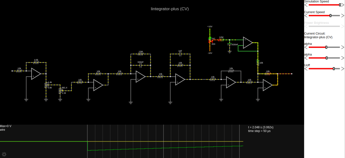
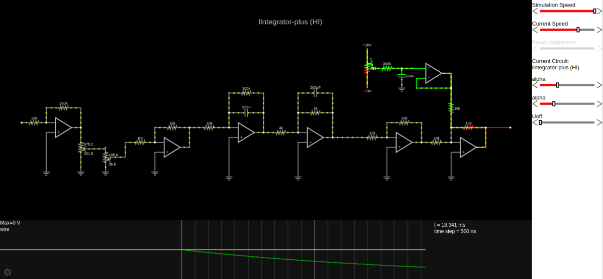
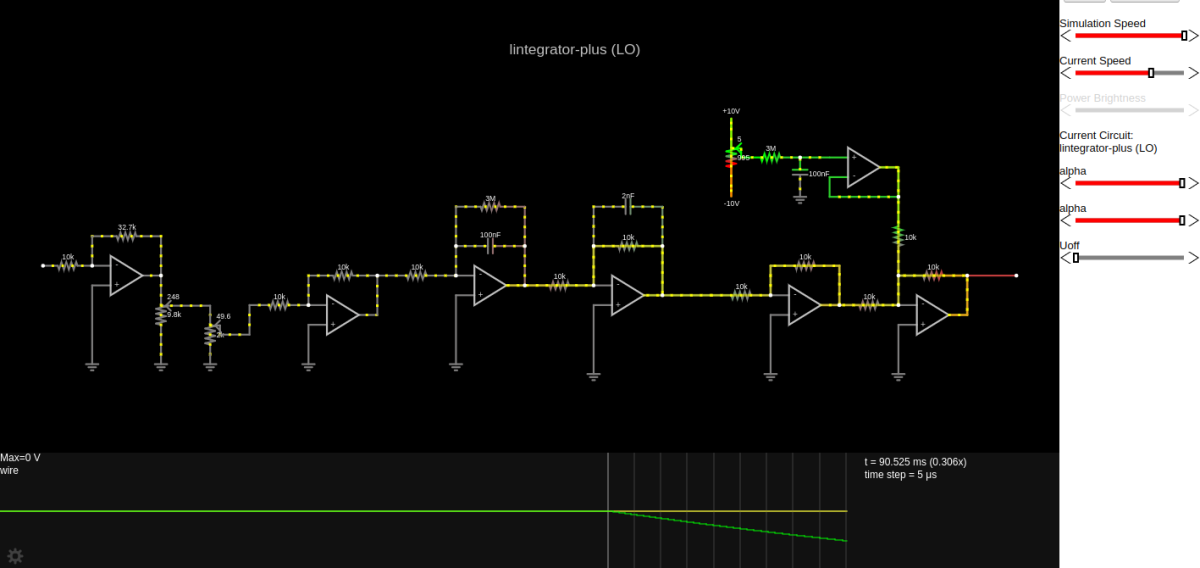
Deze simulaties bevatten ten opzichte van de vorige simulaties zonder Uoff nog een staartje aan de rechter zijde.
Deze simulaties bevatten ten opzichte van de vorige simulaties zonder Uoff nog een staartje aan de rechter zijde.
Hier alvast het schema van het "staartje aan de rechter zijde". Aangezien de weerstand [imath] \mathrm{R}_9 [/imath] voor alle drie de modi (CV, HI en LO) veel groter dan [imath] \mathrm{R}_8 [/imath] is kan de spanning [imath] -\mathrm{U}_{off} [/imath] op nagenoeg lineaire wijze met potmeter [imath] \mathrm{R}_8 [/imath] tussen +10V en -10V ingesteld worden.
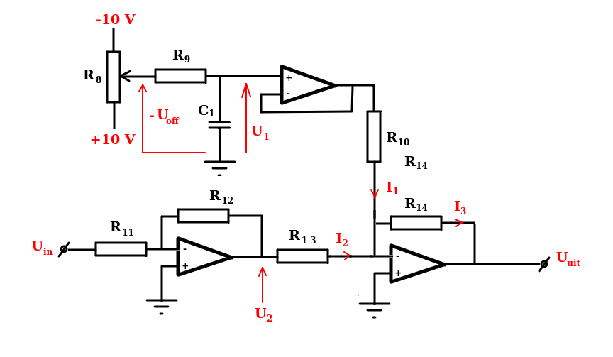
Merk op dat in het schema de -10 V bovenaan staat terwijl in de screen shots van de Falstad simulatie de +10 V bovenaan staat. Dit is omdat de potmeter [imath] \mathrm{R}_8 [/imath] voor [imath] -\mathrm{U}_{off} [/imath] in Falstad op zijn kop staat (wat je ziet door de positie van de loper in het zijpaneeltje te vergelijken met de positie van de loper in de simulatie zelf). De waarden van +10 V en -10 V zijn voor het gemak zo gekozen, maar kunnen in de praktijk nogal afwijken. Ik heb daarvoor zelf bijvoorbeeld een range van ongeveer -10,2V tot +10,9V gemeten. Maar er zitten soms stevige verschillen tussen verschillende exemplaren van dezelfde module. Heel relevant is dat overigens niet zolang de module voor de normalerwijze binnen Eurorack toegestane signaal- en stuurspanningen maar goed werkt.
Merk op dat in het schema de -10 V bovenaan staat terwijl in de screen shots van de Falstad simulatie de +10 V bovenaan staat. Dit is omdat de potmeter [imath] \mathrm{R}_8 [/imath] voor [imath] -\mathrm{U}_{off} [/imath] in Falstad op zijn kop staat (wat je ziet door de positie van de loper in het zijpaneeltje te vergelijken met de positie van de loper in de simulatie zelf). De waarden van +10 V en -10 V zijn voor het gemak zo gekozen, maar kunnen in de praktijk nogal afwijken. Ik heb daarvoor zelf bijvoorbeeld een range van ongeveer -10,2V tot +10,9V gemeten. Maar er zitten soms stevige verschillen tussen verschillende exemplaren van dezelfde module. Heel relevant is dat overigens niet zolang de module voor de normalerwijze binnen Eurorack toegestane signaal- en stuurspanningen maar goed werkt.
Had nog een extra stroom nodig, dus nogmaals:
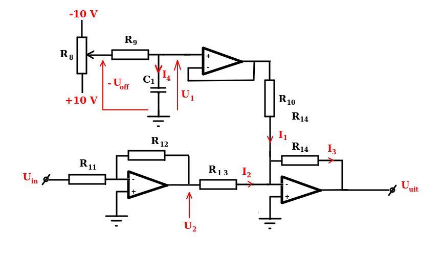
Uit het schema lezen we af:
[imath] I_1 = \frac{ U_1 }{ \mathrm{R}_{10} } \,\,\,\,\,\,\,\,\, (40) [/imath]
[imath] I_2 = \frac{ U_2 }{ \mathrm{R}_{13} } \,\,\,\,\,\,\,\,\, (41) [/imath]
[imath] I_3 = - \frac{ U_{uit} }{ \mathrm{R}_{14} } \,\,\,\,\,\,\,\,\, (42) [/imath]
[imath] I_3 = I_1 + I_2 \,\,\,\,\,\,\,\,\, (43) [/imath]
[imath] I_4 = \mathrm{C}_1 \frac{ \mathrm{d} U_1 }{ \mathrm{d} t } \,\,\,\,\,\,\,\,\, (44) [/imath]
[imath] I_4 = \frac{-\mathrm{U}_{off} \,\, - \,\, U_1}{ \mathrm{R}_9 } \,\,\,\,\,\,\,\,\, (45) [/imath]
[imath] \frac{ U_{in} }{ \mathrm{R}_{11} } = - \frac{ U_2 }{ \mathrm{R}_{12} } \,\,\,\,\,\,\,\,\, (46) [/imath]
Uit de screen shots van de Falstad simulatie zien we bovendien voor alle drie de modi CV, HI en LO dat:
[imath] \mathrm{R}_{11} = \mathrm{R}_{12} \,\,\,\,\,\,\,\,\, (47) [/imath]
[imath] \mathrm{R}_{10} = \mathrm{R}_{13} = \mathrm{R}_{14} \,\,\,\,\,\,\,\,\, (48) [/imath]
Uit het schema lezen we af:
[imath] I_1 = \frac{ U_1 }{ \mathrm{R}_{10} } \,\,\,\,\,\,\,\,\, (40) [/imath]
[imath] I_2 = \frac{ U_2 }{ \mathrm{R}_{13} } \,\,\,\,\,\,\,\,\, (41) [/imath]
[imath] I_3 = - \frac{ U_{uit} }{ \mathrm{R}_{14} } \,\,\,\,\,\,\,\,\, (42) [/imath]
[imath] I_3 = I_1 + I_2 \,\,\,\,\,\,\,\,\, (43) [/imath]
[imath] I_4 = \mathrm{C}_1 \frac{ \mathrm{d} U_1 }{ \mathrm{d} t } \,\,\,\,\,\,\,\,\, (44) [/imath]
[imath] I_4 = \frac{-\mathrm{U}_{off} \,\, - \,\, U_1}{ \mathrm{R}_9 } \,\,\,\,\,\,\,\,\, (45) [/imath]
[imath] \frac{ U_{in} }{ \mathrm{R}_{11} } = - \frac{ U_2 }{ \mathrm{R}_{12} } \,\,\,\,\,\,\,\,\, (46) [/imath]
Uit de screen shots van de Falstad simulatie zien we bovendien voor alle drie de modi CV, HI en LO dat:
[imath] \mathrm{R}_{11} = \mathrm{R}_{12} \,\,\,\,\,\,\,\,\, (47) [/imath]
[imath] \mathrm{R}_{10} = \mathrm{R}_{13} = \mathrm{R}_{14} \,\,\,\,\,\,\,\,\, (48) [/imath]
Uit (46) en (47) zien we dat:
[imath] U_{in} = - U_2 \,\,\,\,\,\,\,\,\, (49) [/imath]
Combinatie van (40), (41), (42) en (43) levert:
[imath] - \frac{ U_{uit} }{ \mathrm{R}_{14} } = \frac{ U_1 }{ \mathrm{R}_{10} } \, + \, \frac{ U_2 }{ \mathrm{R}_{13} } [/imath]
Wat we op basis van (48 ) vereenvoudigen tot:
[imath] - U_{uit} = U_1 \, + \, U_2 \,\,\,\,\,\,\,\,\, (50) [/imath]
Combinatie van (49) en (50) geeft:
[imath] - U_{uit} = U_1 \, + \, - U_{in} [/imath]
[imath] U_1 = U_{in} - U_{uit} \,\,\,\,\,\,\,\,\, (51) [/imath]
Combinatie van (44) en (45) geeft:
[imath] \mathrm{C}_1 \frac{ \mathrm{d} U_1 }{ \mathrm{d} t } = \frac{-\mathrm{U}_{off} \,\, - \,\, U_1}{ \mathrm{R}_9 } [/imath]
[imath] \mathrm{R}_9 \mathrm{C}_1 \cdot \frac{ \mathrm{d} U_1 }{ \mathrm{d} t } = -\mathrm{U}_{off} \,\, - \,\, U_1 \,\,\,\,\,\,\,\,\, (52) [/imath]
Substitutie van (51) in (52) levert:
[imath] \mathrm{R}_9 \mathrm{C}_1 \cdot \frac{ \mathrm{d}}{ \mathrm{d} t } ( U_{in} - U_{uit} ) = -\mathrm{U}_{off} \,\, - \,\, ( U_{in} - U_{uit} ) [/imath]
[imath] \mathrm{R}_9 \mathrm{C}_1 \cdot \frac{ \mathrm{d} U_{in} }{ \mathrm{d} t } \,\, - \,\, \mathrm{R}_9 \mathrm{C}_1 \cdot \frac{ \mathrm{d} U_{uit} }{ \mathrm{d} t } = -\mathrm{U}_{off} \,\, - \,\, U_{in} \, + \, U_{uit} [/imath]
[imath] - \mathrm{R}_9 \mathrm{C}_1 \cdot \frac{ \mathrm{d} U_{in} }{ \mathrm{d} t } \,\, + \,\, \mathrm{R}_9 \mathrm{C}_1 \cdot \frac{ \mathrm{d} U_{uit} }{ \mathrm{d} t } = U_{in} \, - \, U_{uit} \, + \, \mathrm{U}_{off} [/imath]
[imath] \mathrm{R}_9 \mathrm{C}_1 \cdot \frac{ \mathrm{d} U_{uit} }{ \mathrm{d} t } \, + \, U_{uit} = \mathrm{R}_9 \mathrm{C}_1 \cdot \frac{ \mathrm{d} U_{in} }{ \mathrm{d} t } \,\, + \,\,U_{in} \, + \, \mathrm{U}_{off} \,\,\,\,\,\,\,\,\, (53) [/imath]
[imath] U_{in} = - U_2 \,\,\,\,\,\,\,\,\, (49) [/imath]
Combinatie van (40), (41), (42) en (43) levert:
[imath] - \frac{ U_{uit} }{ \mathrm{R}_{14} } = \frac{ U_1 }{ \mathrm{R}_{10} } \, + \, \frac{ U_2 }{ \mathrm{R}_{13} } [/imath]
Wat we op basis van (48 ) vereenvoudigen tot:
[imath] - U_{uit} = U_1 \, + \, U_2 \,\,\,\,\,\,\,\,\, (50) [/imath]
Combinatie van (49) en (50) geeft:
[imath] - U_{uit} = U_1 \, + \, - U_{in} [/imath]
[imath] U_1 = U_{in} - U_{uit} \,\,\,\,\,\,\,\,\, (51) [/imath]
Combinatie van (44) en (45) geeft:
[imath] \mathrm{C}_1 \frac{ \mathrm{d} U_1 }{ \mathrm{d} t } = \frac{-\mathrm{U}_{off} \,\, - \,\, U_1}{ \mathrm{R}_9 } [/imath]
[imath] \mathrm{R}_9 \mathrm{C}_1 \cdot \frac{ \mathrm{d} U_1 }{ \mathrm{d} t } = -\mathrm{U}_{off} \,\, - \,\, U_1 \,\,\,\,\,\,\,\,\, (52) [/imath]
Substitutie van (51) in (52) levert:
[imath] \mathrm{R}_9 \mathrm{C}_1 \cdot \frac{ \mathrm{d}}{ \mathrm{d} t } ( U_{in} - U_{uit} ) = -\mathrm{U}_{off} \,\, - \,\, ( U_{in} - U_{uit} ) [/imath]
[imath] \mathrm{R}_9 \mathrm{C}_1 \cdot \frac{ \mathrm{d} U_{in} }{ \mathrm{d} t } \,\, - \,\, \mathrm{R}_9 \mathrm{C}_1 \cdot \frac{ \mathrm{d} U_{uit} }{ \mathrm{d} t } = -\mathrm{U}_{off} \,\, - \,\, U_{in} \, + \, U_{uit} [/imath]
[imath] - \mathrm{R}_9 \mathrm{C}_1 \cdot \frac{ \mathrm{d} U_{in} }{ \mathrm{d} t } \,\, + \,\, \mathrm{R}_9 \mathrm{C}_1 \cdot \frac{ \mathrm{d} U_{uit} }{ \mathrm{d} t } = U_{in} \, - \, U_{uit} \, + \, \mathrm{U}_{off} [/imath]
[imath] \mathrm{R}_9 \mathrm{C}_1 \cdot \frac{ \mathrm{d} U_{uit} }{ \mathrm{d} t } \, + \, U_{uit} = \mathrm{R}_9 \mathrm{C}_1 \cdot \frac{ \mathrm{d} U_{in} }{ \mathrm{d} t } \,\, + \,\,U_{in} \, + \, \mathrm{U}_{off} \,\,\,\,\,\,\,\,\, (53) [/imath]
Uit de screenshots van de Falstad simulaties vinden we:
Voor CV modus: [imath] \mathrm{R}_9 \mathrm{C}_1 = 12 \mathrm{M} \Omega \cdot 630 \mathrm{nF} = 7,56 \, \mathrm{s} \,\,\,\,\,\,\,\,\, (54) [/imath]
Voor HI modus: [imath] \mathrm{R}_9 \mathrm{C}_1 = 300 \mathrm{k} \Omega \cdot 65 \mathrm{nF} = 19,5 \, \mathrm{ms} \,\,\,\,\,\,\,\,\, (55) [/imath]
Voor LO modus: [imath] \mathrm{R}_9 \mathrm{C}_1 = 3 \mathrm{M} \Omega \cdot 100 \mathrm{nF} = 0,3 \, \mathrm{s} \,\,\,\,\,\,\,\,\, (56) [/imath]
Dus komt [imath] \mathrm{R}_9 \mathrm{C}_1 [/imath] voor de drie modi overeen met de al eerder in (28 ), (29) en (30) gevonden waarden van de tijdsconstante [imath] \tau_2 [/imath] . Bijgevolg mogen we (53) ook schrijven als:
[imath] \tau_2 \, \frac{ \mathrm{d} U_{uit} }{ \mathrm{d} t } \, + \, U_{uit} = \tau_2 \, \frac{ \mathrm{d} U_{in} }{ \mathrm{d} t } \,\, + \,\,U_{in} \, + \, \mathrm{U}_{off} \,\,\,\,\,\,\,\,\, (57) [/imath]
Voor CV modus: [imath] \mathrm{R}_9 \mathrm{C}_1 = 12 \mathrm{M} \Omega \cdot 630 \mathrm{nF} = 7,56 \, \mathrm{s} \,\,\,\,\,\,\,\,\, (54) [/imath]
Voor HI modus: [imath] \mathrm{R}_9 \mathrm{C}_1 = 300 \mathrm{k} \Omega \cdot 65 \mathrm{nF} = 19,5 \, \mathrm{ms} \,\,\,\,\,\,\,\,\, (55) [/imath]
Voor LO modus: [imath] \mathrm{R}_9 \mathrm{C}_1 = 3 \mathrm{M} \Omega \cdot 100 \mathrm{nF} = 0,3 \, \mathrm{s} \,\,\,\,\,\,\,\,\, (56) [/imath]
Dus komt [imath] \mathrm{R}_9 \mathrm{C}_1 [/imath] voor de drie modi overeen met de al eerder in (28 ), (29) en (30) gevonden waarden van de tijdsconstante [imath] \tau_2 [/imath] . Bijgevolg mogen we (53) ook schrijven als:
[imath] \tau_2 \, \frac{ \mathrm{d} U_{uit} }{ \mathrm{d} t } \, + \, U_{uit} = \tau_2 \, \frac{ \mathrm{d} U_{in} }{ \mathrm{d} t } \,\, + \,\,U_{in} \, + \, \mathrm{U}_{off} \,\,\,\,\,\,\,\,\, (57) [/imath]
We hadden al:
[imath] \frac{\mathrm{gn}(\alpha)}{\tau_1} \cdot U_{in} = \tau_3 \cdot \frac{\mathrm{d}^2 U_{out}}{ \mathrm{d} t^2} + \left ( 1 + \frac{\tau_3}{\tau_2} \right ) \cdot \frac{\mathrm{d} U_{out}}{ \mathrm{d} t} + \frac{1}{\tau_2} \cdot U_{out} \,\,\,\,\,\,\, (38) [/imath]
In het geval we ook [imath] \mathrm{U}_{off} [/imath] in onze simulatie meenemen moeten we het "staartje" er nog aan plakken. Voor dit staartje hebben we:
[imath] \tau_2 \, \frac{ \mathrm{d} U_{uit} }{ \mathrm{d} t } \, + \, U_{uit} = \tau_2 \, \frac{ \mathrm{d} U_{in} }{ \mathrm{d} t } \,\, + \,\,U_{in} \, + \, \mathrm{U}_{off} \,\,\,\,\,\,\,\,\, (57) [/imath]
De spanning [imath] U_{out} [/imath] van (38 ) vormt bij toevoeging van het staartje de spanning [imath] U_{in} [/imath] van (57), en dus kunnen we die spanningen dan ook net zo goed met een en het zelfde symbool [imath] U_{bet} [/imath] ("bet" van between) aanduiden. Waardoor (38 ) en (57) overgaan in:
[imath] \frac{\mathrm{gn}(\alpha)}{\tau_1} \cdot U_{in} = \tau_3 \cdot \frac{\mathrm{d}^2 U_{bet}}{ \mathrm{d} t^2} + \left ( 1 + \frac{\tau_3}{\tau_2} \right ) \cdot \frac{\mathrm{d} U_{bet}}{ \mathrm{d} t} + \frac{1}{\tau_2} \cdot U_{bet} \,\,\,\,\,\,\, (58) [/imath]
[imath] \tau_2 \, \frac{ \mathrm{d} U_{uit} }{ \mathrm{d} t } \, + \, U_{uit} = \tau_2 \, \frac{ \mathrm{d} U_{bet} }{ \mathrm{d} t } \,\, + \,\,U_{bet} \, + \, \mathrm{U}_{off} \,\,\,\,\,\,\,\,\, (59) [/imath]
De bedoeling is nu om [imath] U_{bet} [/imath] op de een of andere manier uit deze vergelijkingen te elimineren, we zijn voor het systeem inclusief staartje immers enkel geïnteresseerd in de relatie tussen [imath] U_{in} [/imath] en [imath] U_{uit} [/imath]. Het stelsel vergelijkingen waarmee we voor het systeem inclusief staartje te maken hebben is dus:
[imath] (60) \,\,\,\,\,\,\,\,\, \left \{ \begin{array}{l} \frac{\mathrm{gn}(\alpha)}{\tau_1} \cdot U_{in} = \tau_3 \cdot \frac{\mathrm{d}^2 U_{bet}}{ \mathrm{d} t^2} + \left ( 1 + \frac{\tau_3}{\tau_2} \right ) \cdot \frac{\mathrm{d} U_{bet}}{ \mathrm{d} t} + \frac{1}{\tau_2} \cdot U_{bet} \\ \tau_2 \, \frac{ \mathrm{d} U_{uit} }{ \mathrm{d} t } \, + \, U_{uit} = \tau_2 \, \frac{ \mathrm{d} U_{bet} }{ \mathrm{d} t } \,\, + \,\,U_{bet} \, + \, \mathrm{U}_{off} \end{array} \right . [/imath]
[imath] \frac{\mathrm{gn}(\alpha)}{\tau_1} \cdot U_{in} = \tau_3 \cdot \frac{\mathrm{d}^2 U_{out}}{ \mathrm{d} t^2} + \left ( 1 + \frac{\tau_3}{\tau_2} \right ) \cdot \frac{\mathrm{d} U_{out}}{ \mathrm{d} t} + \frac{1}{\tau_2} \cdot U_{out} \,\,\,\,\,\,\, (38) [/imath]
In het geval we ook [imath] \mathrm{U}_{off} [/imath] in onze simulatie meenemen moeten we het "staartje" er nog aan plakken. Voor dit staartje hebben we:
[imath] \tau_2 \, \frac{ \mathrm{d} U_{uit} }{ \mathrm{d} t } \, + \, U_{uit} = \tau_2 \, \frac{ \mathrm{d} U_{in} }{ \mathrm{d} t } \,\, + \,\,U_{in} \, + \, \mathrm{U}_{off} \,\,\,\,\,\,\,\,\, (57) [/imath]
De spanning [imath] U_{out} [/imath] van (38 ) vormt bij toevoeging van het staartje de spanning [imath] U_{in} [/imath] van (57), en dus kunnen we die spanningen dan ook net zo goed met een en het zelfde symbool [imath] U_{bet} [/imath] ("bet" van between) aanduiden. Waardoor (38 ) en (57) overgaan in:
[imath] \frac{\mathrm{gn}(\alpha)}{\tau_1} \cdot U_{in} = \tau_3 \cdot \frac{\mathrm{d}^2 U_{bet}}{ \mathrm{d} t^2} + \left ( 1 + \frac{\tau_3}{\tau_2} \right ) \cdot \frac{\mathrm{d} U_{bet}}{ \mathrm{d} t} + \frac{1}{\tau_2} \cdot U_{bet} \,\,\,\,\,\,\, (58) [/imath]
[imath] \tau_2 \, \frac{ \mathrm{d} U_{uit} }{ \mathrm{d} t } \, + \, U_{uit} = \tau_2 \, \frac{ \mathrm{d} U_{bet} }{ \mathrm{d} t } \,\, + \,\,U_{bet} \, + \, \mathrm{U}_{off} \,\,\,\,\,\,\,\,\, (59) [/imath]
De bedoeling is nu om [imath] U_{bet} [/imath] op de een of andere manier uit deze vergelijkingen te elimineren, we zijn voor het systeem inclusief staartje immers enkel geïnteresseerd in de relatie tussen [imath] U_{in} [/imath] en [imath] U_{uit} [/imath]. Het stelsel vergelijkingen waarmee we voor het systeem inclusief staartje te maken hebben is dus:
[imath] (60) \,\,\,\,\,\,\,\,\, \left \{ \begin{array}{l} \frac{\mathrm{gn}(\alpha)}{\tau_1} \cdot U_{in} = \tau_3 \cdot \frac{\mathrm{d}^2 U_{bet}}{ \mathrm{d} t^2} + \left ( 1 + \frac{\tau_3}{\tau_2} \right ) \cdot \frac{\mathrm{d} U_{bet}}{ \mathrm{d} t} + \frac{1}{\tau_2} \cdot U_{bet} \\ \tau_2 \, \frac{ \mathrm{d} U_{uit} }{ \mathrm{d} t } \, + \, U_{uit} = \tau_2 \, \frac{ \mathrm{d} U_{bet} }{ \mathrm{d} t } \,\, + \,\,U_{bet} \, + \, \mathrm{U}_{off} \end{array} \right . [/imath]
Goed - hoe verwijderen we [imath] U_{bet} [/imath] ? Is dat überhaupt mogelijk? Laten we startend vanuit (60) zien waar we komen:
[imath] (60) \,\,\,\,\,\,\,\,\, \left \{ \begin{array}{l} \frac{\mathrm{gn}(\alpha)}{\tau_1} \cdot U_{in} = \tau_3 \cdot \frac{\mathrm{d}^2 U_{bet}}{ \mathrm{d} t^2} + \left ( 1 + \frac{\tau_3}{\tau_2} \right ) \cdot \frac{\mathrm{d} U_{bet}}{ \mathrm{d} t} + \frac{1}{\tau_2} \cdot U_{bet} \\ \tau_2 \, \frac{ \mathrm{d} U_{uit} }{ \mathrm{d} t } \, + \, U_{uit} = \tau_2 \, \frac{ \mathrm{d} U_{bet} }{ \mathrm{d} t } \,\, + \,\,U_{bet} \, + \, \mathrm{U}_{off} \end{array} \right . [/imath]
Zodat:
[imath] \left \{ \begin{array}{l} \frac{\mathrm{gn}(\alpha) \, \tau_2 }{\tau_1} \cdot U_{in} = \tau_ 2 \tau_3 \cdot \frac{\mathrm{d}^2 U_{bet}}{ \mathrm{d} t^2} + \left ( \tau_2 + \tau_3 \right ) \cdot \frac{\mathrm{d} U_{bet}}{ \mathrm{d} t} + U_{bet} \\ \tau_2 \, \frac{ \mathrm{d} U_{uit} }{ \mathrm{d} t } \, + \, U_{uit} = \tau_2 \, \frac{ \mathrm{d} U_{bet} }{ \mathrm{d} t } \,\, + \,\,U_{bet} \, + \, \mathrm{U}_{off} \end{array} \right . [/imath]
[imath] \left \{ \begin{array}{l} \frac{\mathrm{gn}(\alpha) \, \tau_2 }{\tau_1} \cdot U_{in} = \tau_ 3 \tau_2 \cdot \frac{\mathrm{d}^2 U_{bet}}{ \mathrm{d} t^2} + \tau_3 \frac{\mathrm{d} U_{bet}}{ \mathrm{d} t} + \tau_2 \frac{\mathrm{d} U_{bet}}{ \mathrm{d} t}+ U_{bet} \\ \tau_2 \, \frac{ \mathrm{d} U_{uit} }{ \mathrm{d} t } \, + \, U_{uit} \, - \, \mathrm{U}_{off}= \tau_2 \, \frac{ \mathrm{d} U_{bet} }{ \mathrm{d} t } \,\, + \,\,U_{bet} \end{array} \right . [/imath]
[imath] \left \{ \begin{array}{l} \frac{\mathrm{gn}(\alpha) \, \tau_2 }{\tau_1} \cdot U_{in} = \tau_ 3 \cdot \left ( \tau_2 \cdot \frac{\mathrm{d}^2 U_{bet}}{ \mathrm{d} t^2} + \frac{\mathrm{d} U_{bet}}{ \mathrm{d} t} \right ) + \tau_2 \frac{\mathrm{d} U_{bet}}{ \mathrm{d} t}+ U_{bet} \\ \tau_2 \, \frac{ \mathrm{d} U_{bet} }{ \mathrm{d} t } \,\, + \,\,U_{bet} \, = \, \tau_2 \, \frac{ \mathrm{d} U_{uit} }{ \mathrm{d} t } \, + \, U_{uit} \, - \, \mathrm{U}_{off} \end{array} \right . [/imath]
[imath] \left \{ \begin{array}{l} \frac{\mathrm{gn}(\alpha) \, \tau_2 }{\tau_1} \cdot U_{in} = \tau_ 3 \cdot \frac{ \mathrm{d} }{ \mathrm{d} t} \left ( \tau_2 \frac{\mathrm{d} U_{bet}}{ \mathrm{d} t} + U_{bet} \right ) + \left ( \tau_2 \frac{\mathrm{d} U_{bet}}{ \mathrm{d} t}+ U_{bet} \right ) \\ \tau_2 \, \frac{ \mathrm{d} U_{bet} }{ \mathrm{d} t } \,\, + \,\,U_{bet} \, = \, \tau_2 \, \frac{ \mathrm{d} U_{uit} }{ \mathrm{d} t } \, + \, U_{uit} \, - \, \mathrm{U}_{off} \end{array} \right . [/imath]
[imath] \frac{\mathrm{gn}(\alpha) \, \tau_2 }{\tau_1} \cdot U_{in} = \tau_ 3 \cdot \frac{ \mathrm{d} }{ \mathrm{d} t} \left ( \tau_2 \, \frac{ \mathrm{d} U_{uit} }{ \mathrm{d} t } \, + \, U_{uit} \, - \, \mathrm{U}_{off} \right ) + \left ( \tau_2 \, \frac{ \mathrm{d} U_{uit} }{ \mathrm{d} t } \, + \, U_{uit} \, - \, \mathrm{U}_{off} \right ) [/imath]
[imath] \frac{\mathrm{gn}(\alpha) \, \tau_2 }{\tau_1} \cdot U_{in} = \tau_ 3 \cdot \left ( \tau_2 \, \frac{ \mathrm{d}^2 U_{uit} }{ \mathrm{d} t^2 } \, + \, \frac{ \mathrm{d} U_{uit} }{ \mathrm{d} t} \, - \, \frac{ \mathrm{d} \mathrm{U}_{off} }{ \mathrm{d} t} \right ) + \tau_2 \, \frac{ \mathrm{d} U_{uit} }{ \mathrm{d} t } \, + \, U_{uit} \, - \, \mathrm{U}_{off} [/imath]
[imath] \frac{\mathrm{gn}(\alpha) \, \tau_2 }{\tau_1} \cdot U_{in} = \tau_ 2 \tau_3 \, \frac{ \mathrm{d}^2 U_{uit} }{ \mathrm{d} t^2 } \, + \, \tau_ 3 \frac{ \mathrm{d} U_{uit} }{ \mathrm{d} t} \, - \, \tau_ 3 \frac{ \mathrm{d} \mathrm{U}_{off} }{ \mathrm{d} t} \, + \, \tau_2 \, \frac{ \mathrm{d} U_{uit} }{ \mathrm{d} t } \, + \, U_{uit} \, - \, \mathrm{U}_{off} [/imath]
[imath] \frac{\mathrm{gn}(\alpha) \, \tau_2 }{\tau_1} \cdot U_{in} \, + \, \tau_ 3 \frac{ \mathrm{d} \mathrm{U}_{off} }{ \mathrm{d} t} \, + \, \mathrm{U}_{off} \, = \, \tau_ 2 \tau_3 \, \frac{ \mathrm{d}^2 U_{uit} }{ \mathrm{d} t^2 } \, + \, \tau_ 3 \frac{ \mathrm{d} U_{uit} }{ \mathrm{d} t} \, + \, \tau_2 \, \frac{ \mathrm{d} U_{uit} }{ \mathrm{d} t } \, + \, U_{uit} [/imath]
[imath] \frac{\mathrm{gn}(\alpha) \, \tau_2 }{\tau_1} \cdot U_{in} \, + \, \tau_ 3 \frac{ \mathrm{d} \mathrm{U}_{off} }{ \mathrm{d} t} \, + \, \mathrm{U}_{off} \, = \, \tau_ 2 \tau_3 \, \frac{ \mathrm{d}^2 U_{uit} }{ \mathrm{d} t^2 } \, + \, ( \tau_2 + \tau_3) \, \frac{ \mathrm{d} U_{uit} }{ \mathrm{d} t } \, + \, U_{uit} \,\,\,\,\,\,\,\,\, (61) [/imath]
Of wanneer we de benadering [imath] \mathrm{gn^*}(\alpha) [/imath] voor [imath] \mathrm{gn}(\alpha) [/imath] gebruiken:
[imath] \frac{\mathrm{gn}^*(\alpha) \, \tau_2 }{\tau_1} \cdot U_{in} \, + \, \tau_ 3 \frac{ \mathrm{d} \mathrm{U}_{off} }{ \mathrm{d} t} \, + \, \mathrm{U}_{off} \, = \, \tau_ 2 \tau_3 \, \frac{ \mathrm{d}^2 U_{uit} }{ \mathrm{d} t^2 } \, + \, ( \tau_2 + \tau_3) \, \frac{ \mathrm{d} U_{uit} }{ \mathrm{d} t } \, + \, U_{uit} \,\,\,\,\,\,\,\,\, (62) [/imath]
[imath] (60) \,\,\,\,\,\,\,\,\, \left \{ \begin{array}{l} \frac{\mathrm{gn}(\alpha)}{\tau_1} \cdot U_{in} = \tau_3 \cdot \frac{\mathrm{d}^2 U_{bet}}{ \mathrm{d} t^2} + \left ( 1 + \frac{\tau_3}{\tau_2} \right ) \cdot \frac{\mathrm{d} U_{bet}}{ \mathrm{d} t} + \frac{1}{\tau_2} \cdot U_{bet} \\ \tau_2 \, \frac{ \mathrm{d} U_{uit} }{ \mathrm{d} t } \, + \, U_{uit} = \tau_2 \, \frac{ \mathrm{d} U_{bet} }{ \mathrm{d} t } \,\, + \,\,U_{bet} \, + \, \mathrm{U}_{off} \end{array} \right . [/imath]
Zodat:
[imath] \left \{ \begin{array}{l} \frac{\mathrm{gn}(\alpha) \, \tau_2 }{\tau_1} \cdot U_{in} = \tau_ 2 \tau_3 \cdot \frac{\mathrm{d}^2 U_{bet}}{ \mathrm{d} t^2} + \left ( \tau_2 + \tau_3 \right ) \cdot \frac{\mathrm{d} U_{bet}}{ \mathrm{d} t} + U_{bet} \\ \tau_2 \, \frac{ \mathrm{d} U_{uit} }{ \mathrm{d} t } \, + \, U_{uit} = \tau_2 \, \frac{ \mathrm{d} U_{bet} }{ \mathrm{d} t } \,\, + \,\,U_{bet} \, + \, \mathrm{U}_{off} \end{array} \right . [/imath]
[imath] \left \{ \begin{array}{l} \frac{\mathrm{gn}(\alpha) \, \tau_2 }{\tau_1} \cdot U_{in} = \tau_ 3 \tau_2 \cdot \frac{\mathrm{d}^2 U_{bet}}{ \mathrm{d} t^2} + \tau_3 \frac{\mathrm{d} U_{bet}}{ \mathrm{d} t} + \tau_2 \frac{\mathrm{d} U_{bet}}{ \mathrm{d} t}+ U_{bet} \\ \tau_2 \, \frac{ \mathrm{d} U_{uit} }{ \mathrm{d} t } \, + \, U_{uit} \, - \, \mathrm{U}_{off}= \tau_2 \, \frac{ \mathrm{d} U_{bet} }{ \mathrm{d} t } \,\, + \,\,U_{bet} \end{array} \right . [/imath]
[imath] \left \{ \begin{array}{l} \frac{\mathrm{gn}(\alpha) \, \tau_2 }{\tau_1} \cdot U_{in} = \tau_ 3 \cdot \left ( \tau_2 \cdot \frac{\mathrm{d}^2 U_{bet}}{ \mathrm{d} t^2} + \frac{\mathrm{d} U_{bet}}{ \mathrm{d} t} \right ) + \tau_2 \frac{\mathrm{d} U_{bet}}{ \mathrm{d} t}+ U_{bet} \\ \tau_2 \, \frac{ \mathrm{d} U_{bet} }{ \mathrm{d} t } \,\, + \,\,U_{bet} \, = \, \tau_2 \, \frac{ \mathrm{d} U_{uit} }{ \mathrm{d} t } \, + \, U_{uit} \, - \, \mathrm{U}_{off} \end{array} \right . [/imath]
[imath] \left \{ \begin{array}{l} \frac{\mathrm{gn}(\alpha) \, \tau_2 }{\tau_1} \cdot U_{in} = \tau_ 3 \cdot \frac{ \mathrm{d} }{ \mathrm{d} t} \left ( \tau_2 \frac{\mathrm{d} U_{bet}}{ \mathrm{d} t} + U_{bet} \right ) + \left ( \tau_2 \frac{\mathrm{d} U_{bet}}{ \mathrm{d} t}+ U_{bet} \right ) \\ \tau_2 \, \frac{ \mathrm{d} U_{bet} }{ \mathrm{d} t } \,\, + \,\,U_{bet} \, = \, \tau_2 \, \frac{ \mathrm{d} U_{uit} }{ \mathrm{d} t } \, + \, U_{uit} \, - \, \mathrm{U}_{off} \end{array} \right . [/imath]
[imath] \frac{\mathrm{gn}(\alpha) \, \tau_2 }{\tau_1} \cdot U_{in} = \tau_ 3 \cdot \frac{ \mathrm{d} }{ \mathrm{d} t} \left ( \tau_2 \, \frac{ \mathrm{d} U_{uit} }{ \mathrm{d} t } \, + \, U_{uit} \, - \, \mathrm{U}_{off} \right ) + \left ( \tau_2 \, \frac{ \mathrm{d} U_{uit} }{ \mathrm{d} t } \, + \, U_{uit} \, - \, \mathrm{U}_{off} \right ) [/imath]
[imath] \frac{\mathrm{gn}(\alpha) \, \tau_2 }{\tau_1} \cdot U_{in} = \tau_ 3 \cdot \left ( \tau_2 \, \frac{ \mathrm{d}^2 U_{uit} }{ \mathrm{d} t^2 } \, + \, \frac{ \mathrm{d} U_{uit} }{ \mathrm{d} t} \, - \, \frac{ \mathrm{d} \mathrm{U}_{off} }{ \mathrm{d} t} \right ) + \tau_2 \, \frac{ \mathrm{d} U_{uit} }{ \mathrm{d} t } \, + \, U_{uit} \, - \, \mathrm{U}_{off} [/imath]
[imath] \frac{\mathrm{gn}(\alpha) \, \tau_2 }{\tau_1} \cdot U_{in} = \tau_ 2 \tau_3 \, \frac{ \mathrm{d}^2 U_{uit} }{ \mathrm{d} t^2 } \, + \, \tau_ 3 \frac{ \mathrm{d} U_{uit} }{ \mathrm{d} t} \, - \, \tau_ 3 \frac{ \mathrm{d} \mathrm{U}_{off} }{ \mathrm{d} t} \, + \, \tau_2 \, \frac{ \mathrm{d} U_{uit} }{ \mathrm{d} t } \, + \, U_{uit} \, - \, \mathrm{U}_{off} [/imath]
[imath] \frac{\mathrm{gn}(\alpha) \, \tau_2 }{\tau_1} \cdot U_{in} \, + \, \tau_ 3 \frac{ \mathrm{d} \mathrm{U}_{off} }{ \mathrm{d} t} \, + \, \mathrm{U}_{off} \, = \, \tau_ 2 \tau_3 \, \frac{ \mathrm{d}^2 U_{uit} }{ \mathrm{d} t^2 } \, + \, \tau_ 3 \frac{ \mathrm{d} U_{uit} }{ \mathrm{d} t} \, + \, \tau_2 \, \frac{ \mathrm{d} U_{uit} }{ \mathrm{d} t } \, + \, U_{uit} [/imath]
[imath] \frac{\mathrm{gn}(\alpha) \, \tau_2 }{\tau_1} \cdot U_{in} \, + \, \tau_ 3 \frac{ \mathrm{d} \mathrm{U}_{off} }{ \mathrm{d} t} \, + \, \mathrm{U}_{off} \, = \, \tau_ 2 \tau_3 \, \frac{ \mathrm{d}^2 U_{uit} }{ \mathrm{d} t^2 } \, + \, ( \tau_2 + \tau_3) \, \frac{ \mathrm{d} U_{uit} }{ \mathrm{d} t } \, + \, U_{uit} \,\,\,\,\,\,\,\,\, (61) [/imath]
Of wanneer we de benadering [imath] \mathrm{gn^*}(\alpha) [/imath] voor [imath] \mathrm{gn}(\alpha) [/imath] gebruiken:
[imath] \frac{\mathrm{gn}^*(\alpha) \, \tau_2 }{\tau_1} \cdot U_{in} \, + \, \tau_ 3 \frac{ \mathrm{d} \mathrm{U}_{off} }{ \mathrm{d} t} \, + \, \mathrm{U}_{off} \, = \, \tau_ 2 \tau_3 \, \frac{ \mathrm{d}^2 U_{uit} }{ \mathrm{d} t^2 } \, + \, ( \tau_2 + \tau_3) \, \frac{ \mathrm{d} U_{uit} }{ \mathrm{d} t } \, + \, U_{uit} \,\,\,\,\,\,\,\,\, (62) [/imath]
De vraag is nu hoe de INIT VALUE dat is: [imath] \mathrm{U}_{init} [/imath] in heel dit verhaal past. Ik heb een aantal opties overwogen maar het simpelste lijkt mij toch om nog een staartje aan de simulatie toe te voegen. Zie onderstaande opzetje:
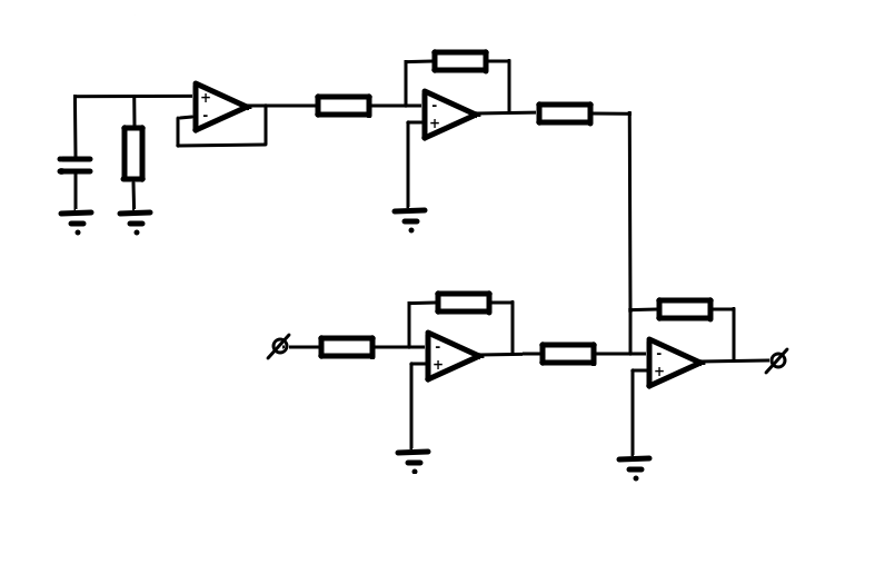
De spanning [imath] \mathrm{U}_{init} [/imath] kan dan in Falstad worden ingesteld door via de "edit..." optie de "Initial Voltage" van de condensator aan te geven.
Morgen verder....
De spanning [imath] \mathrm{U}_{init} [/imath] kan dan in Falstad worden ingesteld door via de "edit..." optie de "Initial Voltage" van de condensator aan te geven.
Morgen verder....
Even terug in de tijd:
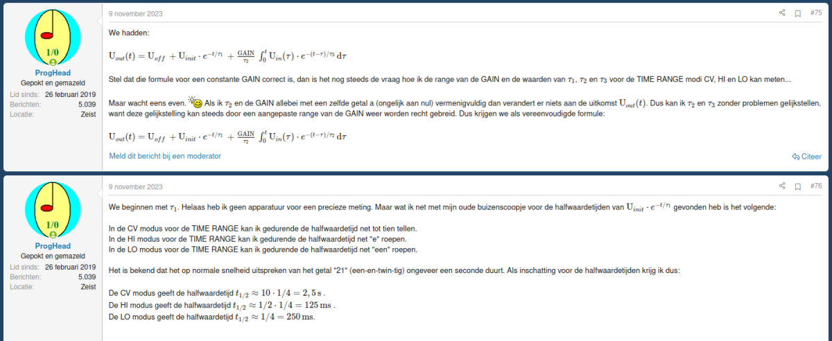
Die formules zijn inmiddels achterhaald, maar de grofweg gemeten halfwaardetijden kunnen we nog goed gebruiken. De uitgangsspanning van de Ladik integrator zal bij [imath] U_{in} = \mathrm{U}_{off} = 0 [/imath] en een positieve INIT VALUE van [imath] \mathrm{U}_{init} [/imath] geleidelijk afnemen, en de tijd waarbij de uitgangsspanning tot de helft (dat is tot [imath] \frac{ \mathrm{U}_{init}}{2} [/imath] ) is afgenomen is de halfwaardetijd [imath] t_{1/2} [/imath]. Voor die halfwaardetijd vonden we zoals we hierboven zien dat:
De CV modus geeft de halfwaardetijd [imath] t_{1/2} \approx 2,5 \, \mathrm{s} \,\,\,\,\,\,\,\,\, (63) [/imath] .
De HI modus geeft de halfwaardetijd [imath] t_{1/2} \approx 125 \, \mathrm{ms} \,\,\,\,\,\,\,\,\, (64)[/imath] .
De LO modus geeft de halfwaardetijd [imath] t_{1/2} \approx 250 \, \mathrm{ms} \,\,\,\,\,\,\,\,\, (65) [/imath].
Die formules zijn inmiddels achterhaald, maar de grofweg gemeten halfwaardetijden kunnen we nog goed gebruiken. De uitgangsspanning van de Ladik integrator zal bij [imath] U_{in} = \mathrm{U}_{off} = 0 [/imath] en een positieve INIT VALUE van [imath] \mathrm{U}_{init} [/imath] geleidelijk afnemen, en de tijd waarbij de uitgangsspanning tot de helft (dat is tot [imath] \frac{ \mathrm{U}_{init}}{2} [/imath] ) is afgenomen is de halfwaardetijd [imath] t_{1/2} [/imath]. Voor die halfwaardetijd vonden we zoals we hierboven zien dat:
De CV modus geeft de halfwaardetijd [imath] t_{1/2} \approx 2,5 \, \mathrm{s} \,\,\,\,\,\,\,\,\, (63) [/imath] .
De HI modus geeft de halfwaardetijd [imath] t_{1/2} \approx 125 \, \mathrm{ms} \,\,\,\,\,\,\,\,\, (64)[/imath] .
De LO modus geeft de halfwaardetijd [imath] t_{1/2} \approx 250 \, \mathrm{ms} \,\,\,\,\,\,\,\,\, (65) [/imath].
De nu ook met een tweede staartje uitgebreide Falstad simulatie van de Ladik integrator geeft voor de CV modus bij [imath] U_{in} = \mathrm{U}_{off} = 0 [/imath] en een positieve INIT VALUE van [imath] \mathrm{U}_{init} = 10 \mathrm{V} [/imath] de halfwaardetijd [imath] t_{1/2} = 2,5 \, \mathrm{s} [/imath]. Dit is in overeenstemming met (63).
Zo ziet het eruit:
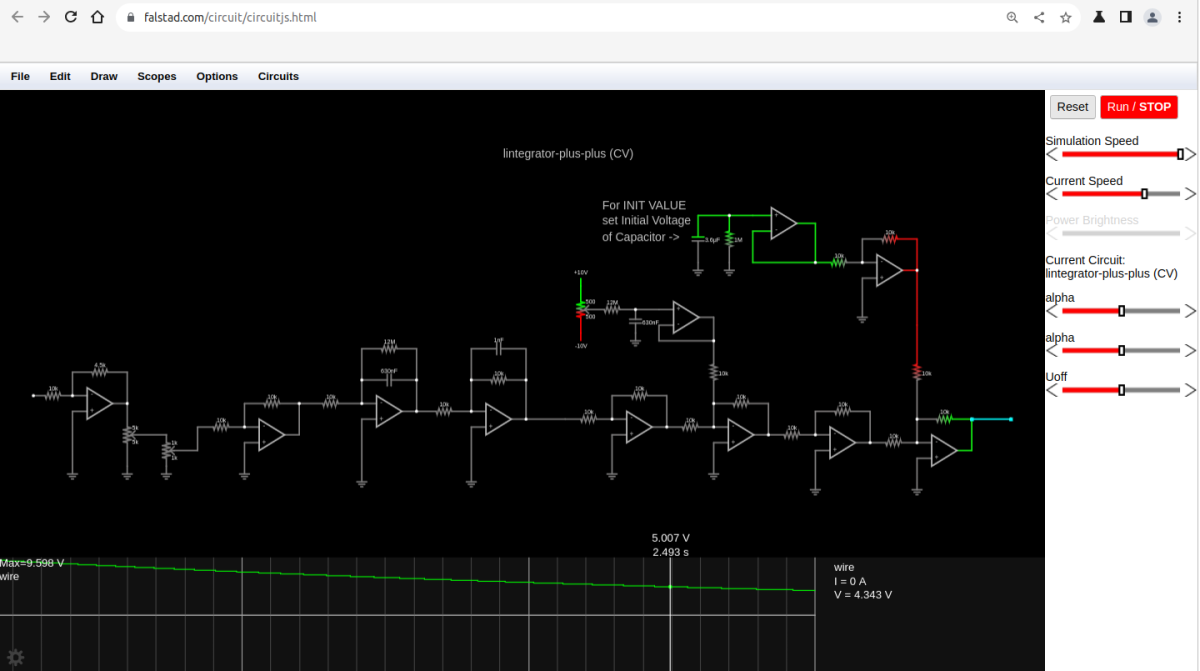
En dit is het Falstad programma:
Zo ziet het eruit:
En dit is het Falstad programma:
Code:
$ 1 0.000049999999999999996 382.76258214399064 69 5 50 5e-11
w 368 -1568 368 -1504 0
w 256 -1568 256 -1504 0
c 256 -1568 368 -1568 0 1e-9 -1.6936921681074053e-30 0
g -448 -1328 -448 -1312 0 0
174 -448 -1328 -368 -1440 1 10000 0.5 alpha
w 144 -1568 144 -1504 0
r 32 -1568 144 -1568 0 12000000
w 368 -1504 368 -1424 0
w 32 -1504 32 -1568 0
w 144 -1504 144 -1440 0
r 256 -1504 368 -1504 0 10000
a 256 -1424 368 -1424 8 15 -15 1000000 -1.6936752313550918e-35 0 100000
g 256 -1408 256 -1296 0 0
r 256 -1440 144 -1440 0 10000
w 256 -1504 256 -1440 0
w 32 -1504 32 -1456 0
r 32 -1456 -96 -1456 0 10000
c 32 -1504 144 -1504 0 6.3e-7 6.586269771918231e-34 0
g 32 -1424 32 -1296 0 0
a 32 -1440 144 -1440 8 15 -15 1000000 6.586203909879132e-39 0 100000
a -560 -1456 -448 -1456 8 15 -15 1000000 -4.1327885748334835e-55 0 100000
a -208 -1392 -96 -1392 8 15 -15 1000000 1.2830351530845381e-48 0 100000
r -560 -1472 -640 -1472 0 10000
r -560 -1520 -448 -1520 0 4500
r -208 -1456 -96 -1456 0 10000
w -560 -1520 -560 -1472 0
w -448 -1520 -448 -1456 0
w -208 -1456 -208 -1408 0
w -96 -1456 -96 -1392 0
g -560 -1440 -560 -1312 0 0
r -208 -1408 -304 -1408 0 10000
g -208 -1376 -208 -1312 0 0
174 -368 -1328 -352 -1376 1 2000 0.5 alpha
g -368 -1328 -368 -1312 0 0
w -352 -1360 -304 -1360 0
w -304 -1360 -304 -1408 0
x 321 -1958 587 -1955 4 24 lintegrator-plus-plus\s(CV)
174 480 -1696 480 -1616 1 1000 0.5 Uoff
r 592 -1648 496 -1648 0 12000000
R 480 -1696 480 -1728 0 0 40 10 0 0 0.5
R 480 -1600 480 -1568 0 0 40 -10 0 0 0.5
c 592 -1648 592 -1600 0 6.3e-7 0.00047459412230231737 0.001
g 592 -1600 592 -1584 0 0
g 544 -1392 544 -1312 0 0
r 544 -1424 448 -1424 0 10000
w 656 -1472 656 -1408 0
w 544 -1472 544 -1424 0
r 544 -1472 656 -1472 0 10000
a 544 -1408 656 -1408 8 15 -15 1000000 5.048684549991726e-30 0 100000
g 752 -1376 752 -1312 0 0
r 752 -1408 656 -1408 0 10000
w 864 -1456 864 -1392 0
w 752 -1456 752 -1408 0
r 752 -1456 864 -1456 0 10000
a 752 -1392 864 -1392 8 15 -15 1000000 4.745751391543786e-9 0 100000
w 368 -1424 448 -1424 0
r 752 -1456 752 -1584 0 10000
a 640 -1632 752 -1632 9 15 -15 1000000 0.00047458937640855323 0.00047459412230231737 100000
w 640 -1616 640 -1584 0
w 640 -1584 752 -1584 0
w 752 -1632 752 -1584 0
w 592 -1648 640 -1648 0
x 524 -1821 705 -1818 4 24 set\sInitial\sVoltage
a 1056 -1728 1168 -1728 8 15 -15 1000000 0.00002090498000791492 0 100000
r 1056 -1792 1168 -1792 0 10000
w 1056 -1792 1056 -1744 0
w 1168 -1792 1168 -1728 0
r 1056 -1744 960 -1744 0 10000
g 1056 -1712 1056 -1632 0 0
x 524 -1853 695 -1850 4 24 For\sINIT\sVALUE
r 1168 -1424 1168 -1616 0 10000
w 720 -1840 784 -1840 0
g 784 -1744 784 -1728 0 0
g 720 -1744 720 -1728 0 0
r 784 -1840 784 -1744 0 1000000
c 720 -1840 720 -1744 0 0.0000036 2.0905607161496147 10
w 1280 -1424 1360 -1424 0
a 1168 -1360 1280 -1360 8 15 -15 1000000 -0.00002089960736321561 0 100000
r 1168 -1424 1280 -1424 0 10000
w 1168 -1424 1168 -1376 0
w 1280 -1424 1280 -1360 0
r 1168 -1376 1072 -1376 0 10000
g 1168 -1344 1168 -1280 0 0
a 960 -1376 1072 -1376 8 15 -15 1000000 -4.745656478414218e-9 0 100000
r 960 -1440 1072 -1440 0 10000
w 960 -1440 960 -1392 0
w 1072 -1440 1072 -1376 0
r 960 -1392 864 -1392 0 10000
g 960 -1360 960 -1280 0 0
w 1168 -1616 1168 -1728 0
a 832 -1824 960 -1824 9 15 -15 1000000 2.090539810751507 2.0905607161496147 100000
w 832 -1808 832 -1744 0
w 832 -1744 960 -1744 0
w 960 -1744 960 -1824 0
w 784 -1840 832 -1840 0
x 524 -1787 682 -1784 4 24 of\sCapacitor\s->
o 76 64 0 4099 20 0.00009765625 0 2 76 3Vergelijkbare discussies

- Reacties
- 73
- Bekeken
- 4K

- Reacties
- 19
- Bekeken
- 950


- Reacties
- 2
- Bekeken
- 1K


- Reacties
- 8
- Bekeken
- 576

Delen: